Tensorflow框架搭建DNN网络训练Mnist数据集

本文将用Tensorflow框架训练Mnist数据集，搭建DNN（深度神经网络），比全连接神经网络多了一些功能，损失将以动态折线图方式展示
Mnist数据集是0-9十个数字构成的图片形式的数据集，每张图片是28*28的大小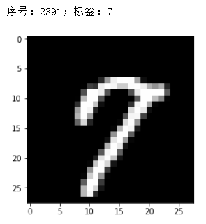
导入tensorflow中带的mnist数据集，以one-hot的形式：

from tensorflow.examples.tutorials.mnist import input_data
mnist=input_data.read_data_sets(".\MNIST_data",one_hot=True)

往神经网络中喂数据的格式是[N,V]结构，整张图片不能直接传入神经网络，每张图片是28乘以28，要变成784*1，即把每个像素挨个排列送进网络

self.x=tf.placeholder(shape=[None,784],dtype=tf.float32)

这里用了三层神经网络，感知机模型f（wx+b），f为激活函数，w为权重，从标准正态分布中截取，b为偏置，设置为0，标准差是0.001

self.w1=tf.Variable(tf.truncated_normal(shape=[784,256],stddev=0.001,dtype=tf.float32))
      self.b1=tf.Variable(tf.zeros(shape=[256],dtype=tf.float32))
      self.w2 = tf.Variable(tf.truncated_normal(shape=[256, 128],stddev=0.001, dtype=tf.float32))
      self.b2 = tf.Variable(tf.zeros(shape=[128], dtype=tf.float32))
      self.w3 = tf.Variable(tf.truncated_normal(shape=[128, 10], stddev=0.001, dtype=tf.float32))
      self.b3 = tf.Variable(tf.zeros(shape=[10], dtype=tf.float32))

这里为了减小计算量，提高训练时间，使用了dropout函数

self.dropout=tf.placeholder(dtype=tf.float32)。。。
dr_y2=tf.nn.dropout(y2,keep_prob=self.dropout)

定义前向通道forward，前两层使用rule作为激活函数，最后一层使用softmax激活（多分类问题最后一层要用softmax激活），并且用batch_normalization做归一化处理

    def forward(self):
        y1=tf.nn.relu(tf.layers.batch_normalization(tf.layers.batch_normalization(tf.matmul(self.x,self.w1)+self.b1)))
        dr_y1=tf.nn.dropout(y1,keep_prob=self.dropout)
        y2=tf.nn.relu(tf.layers.batch_normalization(tf.layers.batch_normalization(tf.matmul(dr_y1,self.w2)+self.b2)))
        dr_y2=tf.nn.dropout(y2,keep_prob=self.dropout)
        self.y3=tf.layers.batch_normalization(tf.matmul(dr_y2,self.w3)+self.b3)
        self.output=tf.nn.softmax(self.y3)

定义损失函数loss,使用交叉熵损失函数softmax_cross_entropy_with_logits，具体用法请自行学习

    def loss(self):
        self.error=tf.reduce_mean(tf.nn.softmax_cross_entropy_with_logits(labels=self.y,logits=self.y3))
        +param*tf.reduce_sum(self.w1**2)+param*tf.reduce_sum(self.w2**2)+param*tf.reduce_sum(self.w3**2)

定义后向函数backward，使用Adam优化器优化损失

    def backfard(self):
        # self.optimizer = tf.train.GradientDescentOptimizer(0.1).minimize(self.error)
        self.optimizer = tf.train.AdamOptimizer(0.001).minimize(self.error)

之后就是主函数，实例化，喂数据，训练、验证，并使用matplotlib将损失以动态折线图的形式展示出来，下面是全部程序

import tensorflow as tf
import numpy as np
from tensorflow.examples.tutorials.mnist import input_data
mnist=input_data.read_data_sets(".\MNIST_data",one_hot=True)
import matplotlib.pyplot as plt
param=1

class Net:
    def __init__(self):
      self.x=tf.placeholder(shape=[None,784],dtype=tf.float32)
      self.y=tf.placeholder(shape=[None,10],dtype=tf.float32)
      self.w1=tf.Variable(tf.truncated_normal(shape=[784,256],stddev=0.001,dtype=tf.float32))
      self.b1=tf.Variable(tf.zeros(shape=[256],dtype=tf.float32))
      self.w2 = tf.Variable(tf.truncated_normal(shape=[256, 128],stddev=0.001, dtype=tf.float32))
      self.b2 = tf.Variable(tf.zeros(shape=[128], dtype=tf.float32))
      self.w3 = tf.Variable(tf.truncated_normal(shape=[128, 10], stddev=0.001, dtype=tf.float32))
      self.b3 = tf.Variable(tf.zeros(shape=[10], dtype=tf.float32))
      self.dropout=tf.placeholder(dtype=tf.float32)
    def forward(self):
        y1=tf.nn.relu(tf.layers.batch_normalization(tf.layers.batch_normalization(tf.matmul(self.x,self.w1)+self.b1)))
        dr_y1=tf.nn.dropout(y1,keep_prob=self.dropout)
        y2=tf.nn.relu(tf.layers.batch_normalization(tf.layers.batch_normalization(tf.matmul(dr_y1,self.w2)+self.b2)))
        dr_y2=tf.nn.dropout(y2,keep_prob=self.dropout)
        self.y3=tf.layers.batch_normalization(tf.matmul(dr_y2,self.w3)+self.b3)
        self.output=tf.nn.softmax(self.y3)

    def loss(self):
        self.error=tf.reduce_mean(tf.nn.softmax_cross_entropy_with_logits(labels=self.y,logits=self.y3))
        +param*tf.reduce_sum(self.w1**2)+param*tf.reduce_sum(self.w2**2)+param*tf.reduce_sum(self.w3**2)
    def backfard(self):
        # self.optimizer = tf.train.GradientDescentOptimizer(0.1).minimize(self.error)
        self.optimizer = tf.train.AdamOptimizer(0.001).minimize(self.error)
    def accuracy(self):
        y=tf.equal(tf.argmax(self.y,axis=1),tf.argmax(self.output,axis=1))
        self.acc=tf.reduce_mean(tf.cast(y,dtype=tf.float32))

if __name__ == '__main__':
    net=Net()
    net.forward()
    net.loss()
    net.backfard()
    net.accuracy()
    init=tf.global_variables_initializer()
    plt.ion()
    a=[]
    b=[]
    c=[]
    with tf.Session() as sess:
        sess.run(init)
        for i in range(50000):
            xs,ys=mnist.train.next_batch(100)
            error,_=sess.run([net.error,net.optimizer],feed_dict={net.x:xs,net.y:ys,net.dropout:0.5})
            if i%100==0:
                xss,yss=mnist.validation.next_batch(100)
                _error,_output,acc=sess.run([net.error,net.output,net.acc],feed_dict={net.x:xss,net.y:yss,net.dropout:1})
                label=np.argmax(yss[0])
                out=np.argmax(_output[0])
                print(acc)
                print("label:",label)
                print("error:",error,"output:",out)
                print("_error:",_error)
                a.append(i)
                b.append(error)
                c.append(_error)
                plt.clf()
                train,=plt.plot(a,b,color="red")
                validation,=plt.plot(a,c,color="blue")
                plt.legend([train,validation],["train","validation"])
                plt.pause(0.01)
    plt.ioff()

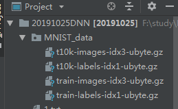
运行之前请确认mnist数据集是否已经加载进来，如果没有要自行下载mnist数据集并粘贴到这里

运行结果：这里不展示动态图，只截取了刚开始运行时的损失和训练一段时间之后的损失
刚开始训练的损失

训练一段时间之后的损失

结论：可以看出，用DNN网络训练mnist数据集，效果还是很好的，毕竟mnist数据集比较简单，比较好训练，最后的损失是很小的。
转载或者引用请注明来源！