一、归一化简介

在对数据进行预处理时，经常要用到归一化方法。

在深度学习中，将数据归一化到一个特定的范围能够在反向传播中获得更好的收敛。如果不进行数据标准化，有些特征（值很大）将会对损失函数影响更大，使得其他值比较小的特征的重要性降低。因此数据标准化可以使得每个特征的重要性更加均衡。

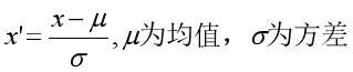
公式表达为：

二、归一化实战

在这里我们可以将上一节所使用的的图像分类的代码，修改为有将数据归一化的代码，命名为 ------ tf_keras_classification_model-normalize，

代码如下：

import进必要的模块

import matplotlib as mpl
import matplotlib.pyplot as plt
#%matplotlib inline
import numpy as np
import sklearn
import pandas as pd

import os
import sys
import time
import tensorflow as tf
from tensorflow import keras

print(tf.__version__)
print(sys.version_info)

for module in mpl,np,pd,sklearn,tf,keras:
    print(module.__name__,module.__version__)

导入数据

# 导入Keras中的数据
fashion_mnist = keras.datasets.fashion_mnist
(x_train_all,y_train_all),(x_test,y_test) = fashion_mnist.load_data()

# 将数据集拆分成训练集与验证集
# 将前5000张图片作为验证集，后55000张图片作为训练集
x_valid,x_train = x_train_all[:5000],x_train_all[5000:]
y_valid,y_train = y_train_all[:5000],y_train_all[5000:]
print(x_valid.shape,y_valid.shape)
print(x_train.shape,y_train.shape)
print(x_test.shape,y_test.shape)

在这里我们可以查看下数据集中的最大最小值

print(np.max(x_train),np.min(x_train))

代码执行结果如下：

255 0

即训练集中最大值为255，最小值为0

接下来我们将数据集中的数据进行归一化处理

from sklearn.preprocessing import StandardScaler
scaler = StandardScaler()
x_train_scaled = scaler.fit_transform(
x_train.astype(np.float32).reshape(-1,1)).reshape(-1,28,28)
x_valid_scaled = scaler.transform(
x_valid.astype(np.float32).reshape(-1,1)).reshape(-1,28,28)
x_test_scaled = scaler.transform(
x_test.astype(np.float32).reshape(-1,1)).reshape(-1,28,28)

在这里 scaler.fit_transform 即是把 x_train 作归一化处理的方法，但这个方法的输入参数要求是二维的，而我们的 x_train 是三维的（[None, 28, 28]）, 故需先将其转化为二维的。

上述 x_train.astype(np.float32).reshape(-1, 1) 的作用就是将三维数据转化为二维（[None, 784]）。

但是在将数据转换为二维进行归一化之后，还需在转化回三维，这样才能传入模型中进行训练。reshape(-1, 28, 28)的作用就是如此。

这里还需注意的是训练集的归一化方法为 scaler.fit_transform，验证集和测试集的归一化方法为scaler.transform。

归一化后我们可以再查看下训练集中的最大最小值：

print(np.max(x_train_scaled),np.min(x_train_scaled))

结果为：

2.0231433 -0.8105136

这样一来将数据归一化处理就做好了。

再构建同样的模型进行训练

model = keras.models.Sequential([
    keras.layers.Flatten(input_shape=[28,28]),
    keras.layers.Dense(300,activation='relu'),
    keras.layers.Dense(100,activation='relu'),
    keras.layers.Dense(10,activation='softmax')
])


#配置学习过程
model.compile(loss = 'sparse_categorical_crossentropy',
             optimizer='sgd',
             metrics=['accuracy'])

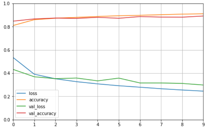
#开启训练
history = model.fit(x_train_scaled,y_train,epochs=10,
                   validation_data=(x_valid_scaled,y_valid))

训练过程打印如下：

Train on 55000 samples, validate on 5000 samples
Epoch 1/10
55000/55000 [==============================] - 10s 175us/sample - loss: 0.5347 - accuracy: 0.8103 - val_loss: 0.4324 - val_accuracy: 0.8478
Epoch 2/10
55000/55000 [==============================] - 8s 149us/sample - loss: 0.3912 - accuracy: 0.8603 - val_loss: 0.3692 - val_accuracy: 0.8670
Epoch 3/10
55000/55000 [==============================] - 15s 273us/sample - loss: 0.3520 - accuracy: 0.8729 - val_loss: 0.3528 - val_accuracy: 0.8742
Epoch 4/10
55000/55000 [==============================] - 11s 195us/sample - loss: 0.3269 - accuracy: 0.8804 - val_loss: 0.3582 - val_accuracy: 0.8714
Epoch 5/10
55000/55000 [==============================] - 10s 185us/sample - loss: 0.3080 - accuracy: 0.8878 - val_loss: 0.3339 - val_accuracy: 0.8806
Epoch 6/10
55000/55000 [==============================] - 11s 202us/sample - loss: 0.2919 - accuracy: 0.8942 - val_loss: 0.3576 - val_accuracy: 0.8726
Epoch 7/10
55000/55000 [==============================] - 7s 136us/sample - loss: 0.2793 - accuracy: 0.8981 - val_loss: 0.3159 - val_accuracy: 0.8872
Epoch 8/10
55000/55000 [==============================] - 8s 149us/sample - loss: 0.2661 - accuracy: 0.9031 - val_loss: 0.3157 - val_accuracy: 0.8828
Epoch 9/10
55000/55000 [==============================] - 9s 166us/sample - loss: 0.2552 - accuracy: 0.9083 - val_loss: 0.3118 - val_accuracy: 0.8820
Epoch 10/10
55000/55000 [==============================] - 8s 152us/sample - loss: 0.2455 - accuracy: 0.9110 - val_loss: 0.2982 - val_accuracy: 0.8920

可以看出相比上一节的训练结果，使用归一化后的训练效果更好。

也可以将训练结果可视化

#变化过程可视化
def plot_learning_curves(history):
    pd.DataFrame(history.history).plot(figsize=(8,5))
    plt.grid(True) #打印网格
    plt.gca().set_ylim(0,1)
    plt.show()
plot_learning_curves(history)

打印结果为：

最后可以对测试集进行评估

#测试，评估
model.evaluate(x_test_scaled,y_test)

输出结果为：

loss: 0.2733 - accuracy: 0.8825

即精度为0.8825

tensorflow2.0学习——tensorflow-keras 归一化

一、归一化简介

二、归一化实战

猜你喜欢