Kaggle数据分析入门之--酒店预订需求

1.需求分析

是否可以根据之前取消的预订情况来预测酒店预订的可能性？

2.数据信息查看和数据清洗

我们使用pandas来查看数据文件，数据文件在https://www.kaggle.com/jessemostipak/hotel-booking-demand，下载一个csv文件。

import pandas as pd
data = pd.read_csv('C:\\Users\\Administrator\\Desktop\\kaggle\\hotel-booking-demand\\hotel_bookings.csv')
data

通过jupyter notebook查看数据信息

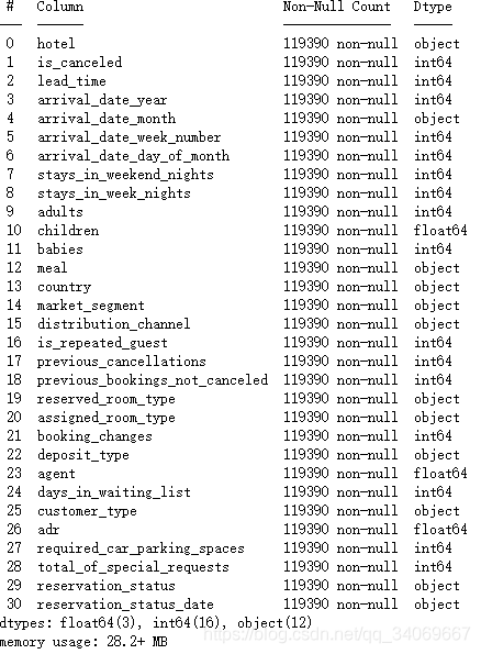
data.info()

<class 'pandas.core.frame.DataFrame'>
RangeIndex: 119390 entries, 0 to 119389
Data columns (total 32 columns):
 #   Column                          Non-Null Count   Dtype  
---  ------                          --------------   -----  
 0   hotel                           119390 non-null  object 
 1   is_canceled                     119390 non-null  int64  
 2   lead_time                       119390 non-null  int64  
 3   arrival_date_year               119390 non-null  int64  
 4   arrival_date_month              119390 non-null  object 
 5   arrival_date_week_number        119390 non-null  int64  
 6   arrival_date_day_of_month       119390 non-null  int64  
 7   stays_in_weekend_nights         119390 non-null  int64  
 8   stays_in_week_nights            119390 non-null  int64  
 9   adults                          119390 non-null  int64  
 10  children                        119386 non-null  float64
 11  babies                          119390 non-null  int64  
 12  meal                            119390 non-null  object 
 13  country                         118902 non-null  object 
 14  market_segment                  119390 non-null  object 
 15  distribution_channel            119390 non-null  object 
 16  is_repeated_guest               119390 non-null  int64  
 17  previous_cancellations          119390 non-null  int64  
 18  previous_bookings_not_canceled  119390 non-null  int64  
 19  reserved_room_type              119390 non-null  object 
 20  assigned_room_type              119390 non-null  object 
 21  booking_changes                 119390 non-null  int64  
 22  deposit_type                    119390 non-null  object 
 23  agent                           103050 non-null  float64
 24  company                         6797 non-null    float64
 25  days_in_waiting_list            119390 non-null  int64  
 26  customer_type                   119390 non-null  object 
 27  adr                             119390 non-null  float64
 28  required_car_parking_spaces     119390 non-null  int64  
 29  total_of_special_requests       119390 non-null  int64  
 30  reservation_status              119390 non-null  object 
 31  reservation_status_date         119390 non-null  object 
dtypes: float64(4), int64(16), object(12)
memory usage: 29.1+ MB

初步分析有32列数据，其中存在有缺失值，有contry、agent等。
接下来对缺失数据进行查看：

data.isnull().sum()[data.isnull().sum()!=0]

children         4
country        488
agent        16340
company     112593
dtype: int64

其中有四项信息存在缺失值，company缺失较多，可以考虑删除，children和country、agent较少，可以考虑填充。

处理方法：

• 假设agent中缺失值代表未指定任何机构，即nan=0
• country则直接使用其字段内众数填充
• childred使用其字段内众数填充
• company因缺失数值过大，且其信息较杂（单个值分布太多），所以直接删除

首先删除company列：

data_new = data.copy(deep = True)
data_new.drop("company", axis=1, inplace=True)

然后对children和country、agent进行填充。
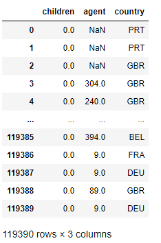
查看children和country、agent的信息

data[['children','agent','country']]

数据插入：

data_new["agent"].fillna(0, inplace=True)
data_new["children"].fillna(data_new["children"].mode()[0], inplace=True)
data_new["country"].fillna(data_new["country"].mode()[0], inplace=True)

再次查看信息：data_new.info()

这里还需要数据异常值的处理：为什么知道这个异常值呢，可以通过后面的计算错误得到这个东西。在后面计算人均价格的时候，如果总人数和为0的情况，则会有异常，所以需要处理异常值
需要对此数据集中异常值为那些总人数（adults+children+babies)为0的记录，同时，因为先前已指名“meal”中“SC”和“Undefined”为同一类别，因此也需要处理一下。

data_new["children"] = data_new["children"].astype(int)
data_new["agent"] = data_new["agent"].astype(int)

data_new["meal"].replace("Undefined", "SC", inplace=True)
# 处理异常值
# 将 变量 adults + children + babies == 0 的数据删除
zero_guests = list(data_new["adults"] +
                  data_new["children"] +
                  data_new["babies"] == 0)
# hb_new.info()
data_new.drop(data_new.index[zero_guests], inplace=True)

3.数据分析(数据可视化)

因为是酒店的需求分析，那我们需要去寻找各个属性之间的关系，以及与结果之间(是否取消)的关系。
我们首先看一下入住率和取消数。

3.1入住率和取消数

fig = plt.figure()
fig.set(alpha=0.2)  # 设定图表颜色alpha参数
data_new.is_canceled.value_counts().plot(kind='bar')# 柱状图 
plt.title(u"取消预订情况 (1为取消预订)") # 标题
plt.ylabel(u"酒店数")  
cancel = data_new.is_canceled.value_counts()
Sum=cancel.sum()
count=0
for i in cancel:   # 显示百分比
    plt.text(count,i+0.5, str('{:.2f}'.format(cancel[count]/Sum *100)) +'%', \
    ha='center') #位置，高度，内容，居中
    count= count + 1
plt.show()

可以看出取消率为37%，入住率为63%左右。
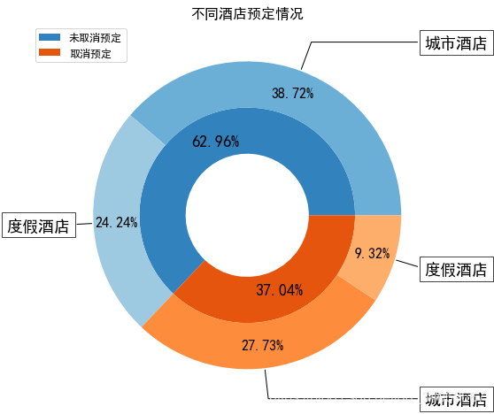
这只是一个基本分析，然后查看不同酒店的入住率与取消率。

rh_iscancel_count = data_new[data_new["hotel"]=="Resort Hotel"].groupby(["is_canceled"])["is_canceled"].count()
ch_iscancel_count = data_new[data_new["hotel"]=="City Hotel"].groupby(["is_canceled"])["is_canceled"].count()

rh_cancel_data = pd.DataFrame({"hotel": "度假酒店",
                              "is_canceled": rh_iscancel_count.index,
                              "count": rh_iscancel_count.values})

ch_cancel_data = pd.DataFrame({"hotel": "城市酒店",
                              "is_canceled": ch_iscancel_count.index,
                              "count": ch_iscancel_count.values})
iscancel_data = pd.concat([rh_cancel_data, ch_cancel_data], ignore_index=True)
plt.figure(figsize=(12, 8))

cmap = plt.get_cmap("tab20c")
outer_colors = cmap(np.arange(2)*4)
inner_colors = cmap(np.array([1, 2, 5, 6]))

w , t, at = plt.pie(hb_new["is_canceled"].value_counts(), autopct="%.2f%%",textprops={"fontsize":18},
                   radius=0.7, wedgeprops=dict(width=0.3), pctdistance=0.75, colors=outer_colors)
plt.legend(w, ["未取消预定", "取消预定"], loc="upper right", bbox_to_anchor=(0, 0, 0.2, 1), fontsize=12)


val_array = np.array((iscancel_data.loc[(iscancel_data.hotel=="城市酒店")&(iscancel_data.is_canceled==0), "count"].values,
       iscancel_data.loc[(iscancel_data.hotel=="度假酒店")&(iscancel_data.is_canceled==0), "count"].values,
       iscancel_data.loc[(iscancel_data.hotel=="城市酒店")&(iscancel_data.is_canceled==1), "count"].values,
       iscancel_data.loc[(iscancel_data.hotel=="度假酒店")&(iscancel_data.is_canceled==1), "count"].values))

w2, t2, at2 = plt.pie(val_array, autopct="%.2f%%",textprops={"fontsize":16}, radius=1,
       wedgeprops=dict(width=0.3), pctdistance=0.85, colors=inner_colors)
plt.title("不同酒店预定情况", fontsize=16)

bbox_props = dict(boxstyle="square,pad=0.3", fc="w", ec="k", lw=0.72)
kw = dict(arrowprops=dict(arrowstyle="-", color="k"), bbox=bbox_props, zorder=3, va="center")
for i, p in enumerate(w2):
#     print(i, p, sep="---")
    text = ["城市酒店", "度假酒店", "城市酒店", "度假酒店"]
    ang = (p.theta2 - p.theta1) / 2. + p.theta1
    y = np.sin(np.deg2rad(ang))
    x = np.cos(np.deg2rad(ang))
    horizontalalignment = {-1: "right", 1: "left"}[int(np.sign(x))]
    connectionstyle = "angle, angleA=0, angleB={}".format(ang)
    kw["arrowprops"].update({"connectionstyle": connectionstyle})
    plt.annotate(text[i], xy=(x, y), xytext=(1.15*np.sign(x), 1.2*y),
                horizontalalignment=horizontalalignment, **kw, fontsize=18)

3.2 酒店人均价格

接下来可以从人均价格入手，看看两家酒店的运营情况。

因为babies年龄过小，所以人均价格中未将babies带入计算。
$人均价格/晚 = \frac{adr}{adults+children}$

此时来查看不同月份下的平均酒店价格，代码如下：

data_new["adr_pp"] = data_new["adr"] / (data_new["adults"] + data_new["children"])
full_data_guests = data_new.loc[data_new["is_canceled"] == 0] # only actual gusts
room_prices = full_data_guests[["hotel", "reserved_room_type", "adr_pp"]].sort_values("reserved_room_type")
room_price_monthly = full_data_guests[["hotel", "arrival_date_month", "adr_pp"]].sort_values("arrival_date_month")

ordered_months = ["January", "February", "March", "April", "May", "June", "July", "August",
                 "September", "October", "November", "December"]
month_che = ["一月", "二月", "三月", "四月", "五月", "六月", "七月", "八月", "九月", "十月", "十一月", "十二月", ]

for en, che in zip(ordered_months, month_che):
    room_price_monthly["arrival_date_month"].replace(en, che, inplace=True)
room_price_monthly["arrival_date_month"] = pd.Categorical(room_price_monthly["arrival_date_month"],
                                                         categories=month_che, ordered=True)
room_price_monthly["hotel"].replace("City Hotel", "城市酒店", inplace=True)
room_price_monthly["hotel"].replace("Resort Hotel", "度假酒店", inplace=True)
room_price_monthly.head(15)

plt.figure(figsize=(12, 8))
sns.lineplot(x="arrival_date_month", y="adr_pp", hue="hotel", data=room_price_monthly,
            hue_order=["城市酒店", "度假酒店"], ci="sd", size="hotel", sizes=(2.5, 2.5))
plt.title("不同月份人均居住价格/晚", fontsize=16)
plt.xlabel("月份", fontsize=16)
plt.ylabel("人均居住价格/晚", fontsize=16)
# plt.savefig("F:/文章/不同月份人均居住价格每晚")

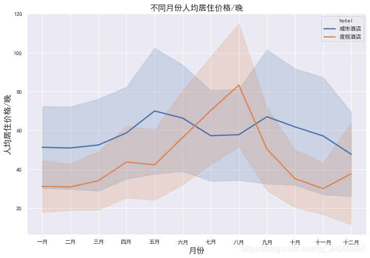
这里可以看到处理异常值的必要性，否则会出现错误。

3.3查看月度人流量

# 查看月度人流量
rh_bookings_monthly = full_data_guests[full_data_guests.hotel=="Resort Hotel"].groupby("arrival_date_month")["hotel"].count()
ch_bookings_monthly = full_data_guests[full_data_guests.hotel=="City Hotel"].groupby("arrival_date_month")["hotel"].count()

rh_bookings_data = pd.DataFrame({"arrival_date_month": list(rh_bookings_monthly.index),
                                "hotel": "度假酒店",
                                "guests": list(rh_bookings_monthly.values)})
ch_bookings_data = pd.DataFrame({"arrival_date_month": list(ch_bookings_monthly.index),
                                "hotel": "城市酒店",
                                "guests": list(ch_bookings_monthly.values)})
full_booking_monthly_data = pd.concat([rh_bookings_data, ch_bookings_data], ignore_index=True)

ordered_months = ["January", "February", "March", "April", "May", "June", "July", "August",
                 "September", "October", "November", "December"]
month_che = ["一月", "二月", "三月", "四月", "五月", "六月", "七月", "八月", "九月", "十月", "十一月", "十二月"]

for en, che in zip(ordered_months, month_che):
    full_booking_monthly_data["arrival_date_month"].replace(en, che, inplace=True)

full_booking_monthly_data["arrival_date_month"] = pd.Categorical(full_booking_monthly_data["arrival_date_month"],
                                                      categories=month_che, ordered=True)

full_booking_monthly_data.loc[(full_booking_monthly_data["arrival_date_month"]=="七月")|\
                             (full_booking_monthly_data["arrival_date_month"]=="八月"), "guests"] /= 3
full_booking_monthly_data.loc[~((full_booking_monthly_data["arrival_date_month"]=="七月")|\
                             (full_booking_monthly_data["arrival_date_month"]=="八月")), "guests"] /= 2
plt.figure(figsize=(12, 8))
sns.lineplot(x="arrival_date_month",
            y="guests",
            hue="hotel", hue_order=["城市酒店", "度假酒店"],
            data=full_booking_monthly_data, size="hotel", sizes=(2.5, 2.5))
plt.title("不同月份平均旅客数", fontsize=16)
plt.xlabel("月份", fontsize=16)
plt.ylabel("旅客数", fontsize=16)
# plt.savefig("F:/文章/不同月份平均旅客数")

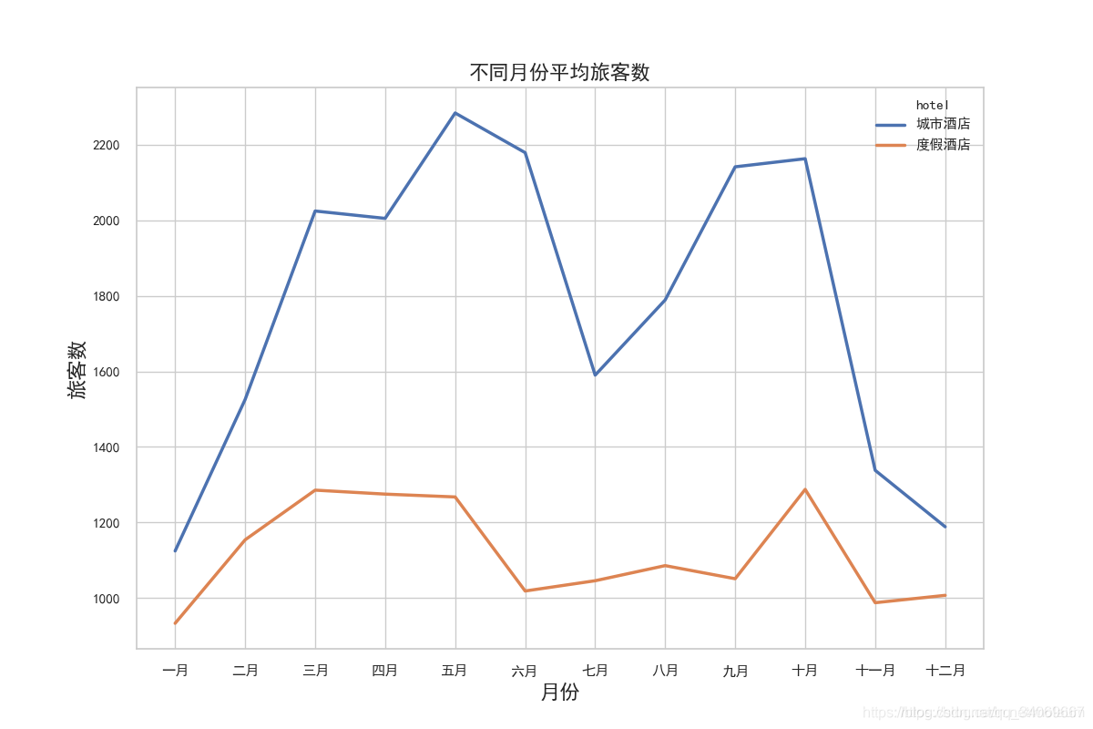
结合上述两幅图可以了解到：

在春秋两季城市酒店价格虽然高，但其入住人数一点也没降低，反而处于旺季；
而度假酒店在6-9月份游客数本身就偏低，可这个时间段内的价格却在持续上升，远高于其他月份；
不论是城市酒店还是度假酒店，冬季的生意都不是特别好。

3.4餐食选择

meal_data = data_new[["hotel", "is_canceled", "meal"]]
# meal_data

plt.figure(figsize=(12, 8))
plt.subplot(121)
plt.pie(meal_data.loc[meal_data["is_canceled"]==0, "meal"].value_counts(), 
        labels=meal_data.loc[meal_data["is_canceled"]==0, "meal"].value_counts().index, 
       autopct="%.2f%%")
plt.title("未取消预订旅客餐食选择", fontsize=16)
plt.legend(loc="upper right")

plt.subplot(122)
plt.pie(meal_data.loc[meal_data["is_canceled"]==1, "meal"].value_counts(), 
        labels=meal_data.loc[meal_data["is_canceled"]==1, "meal"].value_counts().index, 
       autopct="%.2f%%")
plt.title("取消预订旅客餐食选择", fontsize=16)
plt.legend(loc="upper right")

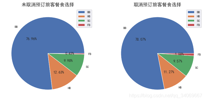
很明显，取消预订旅客和未取消预订旅客有基本相同的餐食选择，所以此特征在后面可以删掉。

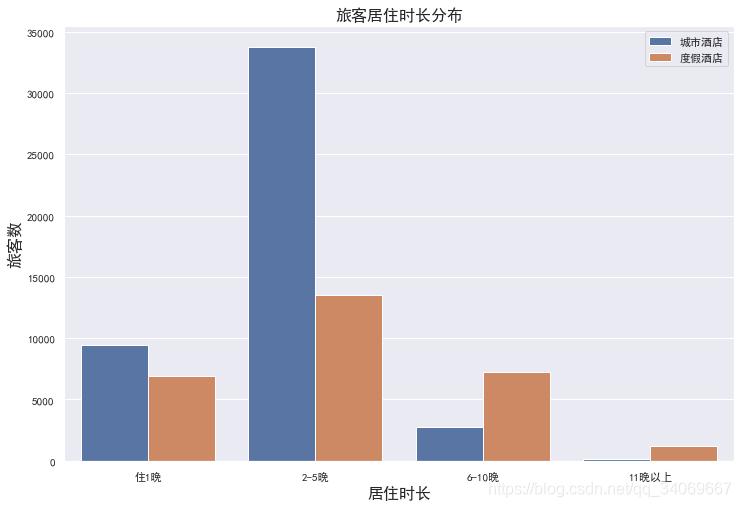
3.5居住时长

那么在不同酒店居住的旅客通常会选择住几天呢？我们可以使用柱形图来看一下其时长的不同分布；

首先计算出总时长：总时长=周末停留夜晚数+工作日停留夜晚数

full_data_guests["total_nights"] = full_data_guests["stays_in_weekend_nights"] + full_data_guests["stays_in_week_nights"]

# 新建字段：total_nights_bin——居住时长区间
full_data_guests["total_nights_bin"] = "住1晚"
full_data_guests.loc[(full_data_guests["total_nights"]>1)&(full_data_guests["total_nights"]<=5), "total_nights_bin"] = "2-5晚"
full_data_guests.loc[(full_data_guests["total_nights"]>5)&(full_data_guests["total_nights"]<=10), "total_nights_bin"] = "6-10晚"
full_data_guests.loc[(full_data_guests["total_nights"]>10), "total_nights_bin"] = "11晚以上"

ch_nights_count = full_data_guests["total_nights_bin"][full_data_guests.hotel=="City Hotel"].value_counts()
rh_nights_count = full_data_guests["total_nights_bin"][full_data_guests.hotel=="Resort Hotel"].value_counts()

ch_nights_index = full_data_guests["total_nights_bin"][full_data_guests.hotel=="City Hotel"].value_counts().index
rh_nights_index = full_data_guests["total_nights_bin"][full_data_guests.hotel=="Resort Hotel"].value_counts().index

ch_nights_data = pd.DataFrame({"hotel": "城市酒店",
                               "nights": ch_nights_index,
                              "guests": ch_nights_count})
rh_nights_data = pd.DataFrame({"hotel": "度假酒店",
                               "nights": rh_nights_index,
                              "guests": rh_nights_count})
# 绘图数据
nights_data = pd.concat([ch_nights_data, rh_nights_data], ignore_index=True)
order = ["住1晚", "2-5晚", "6-10晚", "11晚以上"]
nights_data["nights"] = pd.Categorical(nights_data["nights"], categories=order, ordered=True)

plt.figure(figsize=(12, 8))
sns.barplot(x="nights", y="guests", hue="hotel", data=nights_data)
plt.title("旅客居住时长分布", fontsize=16)
plt.xlabel("居住时长", fontsize=16)
plt.ylabel("旅客数", fontsize=16)

plt.legend()

3.6提前预定时长

提前预定期对旅客是否选择取消预订也有很大影响，因为lead_time字段中的值分布多且散乱，所以使用散点图比较合适，同时还可以绘制一条回归线。

lead_cancel_data = pd.DataFrame(data_new.groupby("lead_time")["is_canceled"].describe())
# lead_cancel_data
# 因为lead_time中值范围大且数量分布不匀，所以选取lead_time>10次的数据（<10的数据不具代表性）
lead_cancel_data_10 = lead_cancel_data[lead_cancel_data["count"]>10]

y = list(round(lead_cancel_data_10["mean"], 4) * 100)

plt.figure(figsize=(12, 8))
sns.regplot(x=list(lead_cancel_data_10.index),
           y=y)
plt.title("提前预定时长对取消的影响", fontsize=16)
plt.xlabel("提前预定时长", fontsize=16)
plt.ylabel("取消数 [%]", fontsize=16)
# plt.savefig("F:/文章/提前预定时长对取消的影响")

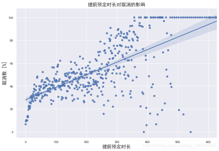
可以明显看到：不同的提前预定时长确定对旅客是否取消预定有一定影响；

通常，越早预订，越容易取消酒店房间预定。

4.进行各属性的分辨，哪个更重要

可以利用data.corr()进行相关性的判断 #相关系数矩阵，即给出了任意两个变量之间的相关系数

cancel_corr = data_new.corr()["is_canceled"]
cancel_corr.abs().sort_values(ascending=False)[1:]

lead_time                         0.292876
total_of_special_requests         0.234877
required_car_parking_spaces       0.195701
booking_changes                   0.144832
previous_cancellations            0.110139
is_repeated_guest                 0.083745
adults                            0.058182
previous_bookings_not_canceled    0.057365
days_in_waiting_list              0.054301
agent                             0.046770
adr                               0.046492
babies                            0.032569
stays_in_week_nights              0.025542
adr_pp                            0.017808
arrival_date_year                 0.016622
arrival_date_week_number          0.008315
arrival_date_day_of_month         0.005948
children                          0.004851
stays_in_weekend_nights           0.001323

从上表中可以看到lead_time、total_of_special_requests 、required_car_parking_spaces、booking_changes 、previous_cancellations这五个特征影响最大。
这里需要对特征进行判断，哪些不必要，哪些是必要的。还有哪些特征我们没有包含，因为部分特征并不是以数值方式显示，所以在进行相关计算时，不能计算，这时我们也要考虑这些特征，比如"reservation_status"（预订状态），这个我们应当考虑。
来查看一下这个特征：

data_new.groupby("is_canceled")["reservation_status"].value_counts()

is_canceled  reservation_status
0            Check-Out             75011
1            Canceled              42993
             No-Show                1206

可以看到退房和取消的数目，还有没有展示的少数。

5.特征模型训练

好了，那我们接下来就用以下特征作为模型数据：
当然，你可以选择其他的特征，或者少一部分特征，这个是可以的，因为模型的最优都要经过调试和试验，没有第一次就最好的。按照吴恩达老师，首先弄一个base model，看一下效果如何。
先用python的各个机器学习算法进行试验一下准确率。
比如决策树、随机森林、逻辑回归、XGBC分类器等
首先导入需要的机器学习的包：

# for ML:
from sklearn.model_selection import train_test_split, KFold, cross_validate, cross_val_score
from sklearn.pipeline import Pipeline
from sklearn.compose import ColumnTransformer
from sklearn.preprocessing import LabelEncoder, OneHotEncoder
from sklearn.impute import SimpleImputer
from sklearn.ensemble import RandomForestClassifier  # 随机森林
from xgboost import XGBClassifier 
from sklearn.linear_model import LogisticRegression
from sklearn.tree import DecisionTreeClassifier
from sklearn.metrics import accuracy_score
import eli5 # Feature importance evaluation

#手动选择要包括的列
#为了使模型更通用并防止泄漏，排除了一些列
#（到达日期、年份、指定房间类型、预订更改、预订状态、国家/地区，
#等待日列表）
#包括国家将提高准确性，但它也可能使模型不那么通用
num_features = ["lead_time","arrival_date_week_number","arrival_date_day_of_month",
                "stays_in_weekend_nights","stays_in_week_nights","adults","children",
                "babies","is_repeated_guest", "previous_cancellations",
                "previous_bookings_not_canceled","agent",
                "required_car_parking_spaces", "total_of_special_requests", "adr"]

cat_features = ["hotel","arrival_date_month","meal","market_segment",
                "distribution_channel","reserved_room_type","deposit_type","customer_type"]
#分离特征和预测值
features = num_features + cat_features
X = data_new.drop(["is_canceled"], axis=1)[features]
y = data_new["is_canceled"]

#预处理数值特征：
#对于大多数num cols，除了日期，0是最符合逻辑的填充值
#这里没有日期遗漏。
num_transformer = SimpleImputer(strategy="constant")

# 分类特征的预处理：
cat_transformer = Pipeline(steps=[
    ("imputer", SimpleImputer(strategy="constant", fill_value="Unknown")),
    ("onehot", OneHotEncoder(handle_unknown='ignore'))])

# 数值和分类特征的束预处理：
preprocessor = ColumnTransformer(transformers=[("num", num_transformer, num_features),
                                               ("cat", cat_transformer, cat_features)])

# 定义要测试的模型：
base_models = [("DT_model", DecisionTreeClassifier(random_state=42)),
               ("RF_model", RandomForestClassifier(random_state=42,n_jobs=-1)),
               ("LR_model", LogisticRegression(random_state=42,n_jobs=-1)),
               ("XGB_model", XGBClassifier(random_state=42, n_jobs=-1))]

#将数据分成“kfold”部分进行交叉验证，
#使用shuffle确保数据的随机分布：
kfolds = 4 # 4 = 75% train, 25% validation
split = KFold(n_splits=kfolds, shuffle=True, random_state=42)

#对每个模型进行预处理、拟合、预测和评分：
for name, model in base_models:
    #将数据和模型的预处理打包到管道中：
    model_steps = Pipeline(steps=[('preprocessor', preprocessor),
                              ('model', model)])
    
    #获取每个模型的交叉验证分数：
    cv_results = cross_val_score(model_steps, 
                                 X, y, 
                                 cv=split,
                                 scoring="accuracy",
                                 n_jobs=-1)
    # output:
    min_score = round(min(cv_results), 4)
    max_score = round(max(cv_results), 4)
    mean_score = round(np.mean(cv_results), 4)
    std_dev = round(np.std(cv_results), 4)
    print(f"{name} cross validation accuarcy score: {mean_score} +/- {std_dev} (std) min: {min_score}, max: {max_score}")

结果：

DT_model cross validation accuarcy score: 0.8255 +/- 0.0012 (std) min: 0.8241, max: 0.827
RF_model cross validation accuarcy score: 0.8663 +/- 0.0005 (std) min: 0.8653, max: 0.8667
LR_model cross validation accuarcy score: 0.7956 +/- 0.0017 (std) min: 0.7941, max: 0.7983
XGB_model cross validation accuarcy score: 0.8465 +/- 0.0008 (std) min: 0.8452, max: 0.8474

可以看到采用随机森林RF_model的效果最好。
你可以继续对其进行一些超参数的优化。

# Enhanced RF model with the best parameters I found:
rf_model_enh = RandomForestClassifier(n_estimators=160,
                               max_features=0.4,
                               min_samples_split=2,
                               n_jobs=-1,
                               random_state=0)

split = KFold(n_splits=kfolds, shuffle=True, random_state=42)
model_pipe = Pipeline(steps=[('preprocessor', preprocessor),
                              ('model', rf_model_enh)])
cv_results = cross_val_score(model_pipe, 
                                 X, y, 
                                 cv=split,
                                 scoring="accuracy",
                                 n_jobs=-1)
# output:
min_score = round(min(cv_results), 4)
max_score = round(max(cv_results), 4)
mean_score = round(np.mean(cv_results), 4)
std_dev = round(np.std(cv_results), 4)
print(f"Enhanced RF model cross validation accuarcy score: {mean_score} +/- {std_dev} (std) min: {min_score}, max: {max_score}")

Enhanced RF model cross validation accuarcy score: 0.8677 +/- 0.002 (std) min: 0.8644, max: 0.8694
可以看到精度有适当提高。

6.评价特征的重要性

#拟合模型，以便可以访问值：
model_pipe.fit(X,y)

#需要所有（编码）功能的名称。
#从一个热编码中获取列的名称：
onehot_columns = list(model_pipe.named_steps['preprocessor'].
                      named_transformers_['cat'].
                      named_steps['onehot'].
                      get_feature_names(input_features=cat_features))

#为完整列表添加num_功能。
#顺序必须与X的定义相同，其中num_特征是第一个：
feat_imp_list = num_features + onehot_columns

#显示10个最重要的功能，提供功能名称：
feat_imp_df = eli5.formatters.as_dataframe.explain_weights_df(
    model_pipe.named_steps['model'],
    feature_names=feat_imp_list)
feat_imp_df.head(10)

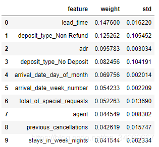
查看三个最重要的功能：

• lead_time
• deposit_type
• adr

lead_time的功能

# group data for lead_time:
lead_cancel_data = data_new.groupby("lead_time")["is_canceled"].describe()
# use only lead_times wih more than 10 bookings for graph:
lead_cancel_data_10 = lead_cancel_data.loc[lead_cancel_data["count"] >= 10]

#show figure:
plt.figure(figsize=(12, 8))
sns.regplot(x=lead_cancel_data_10.index, y=lead_cancel_data_10["mean"].values * 100)
plt.title("Effect of lead time on cancelation", fontsize=16)
plt.xlabel("Lead time", fontsize=16)
plt.ylabel("Cancelations [%]", fontsize=16)
# plt.xlim(0,365)
plt.show()

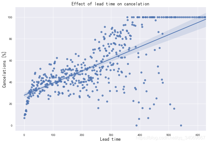
在到达日期前几天进行的预订很少被取消，而提前一年以上的预订则经常被取消。

存款类型：

# group data for deposit_type:
deposit_cancel_data = data_new.groupby("deposit_type")["is_canceled"].describe()

#show figure:
plt.figure(figsize=(12, 8))
sns.barplot(x=deposit_cancel_data.index, y=deposit_cancel_data["mean"] * 100)
plt.title("Effect of deposit_type on cancelation", fontsize=16)
plt.xlabel("Deposit type", fontsize=16)
plt.ylabel("Cancelations [%]", fontsize=16)
plt.show()

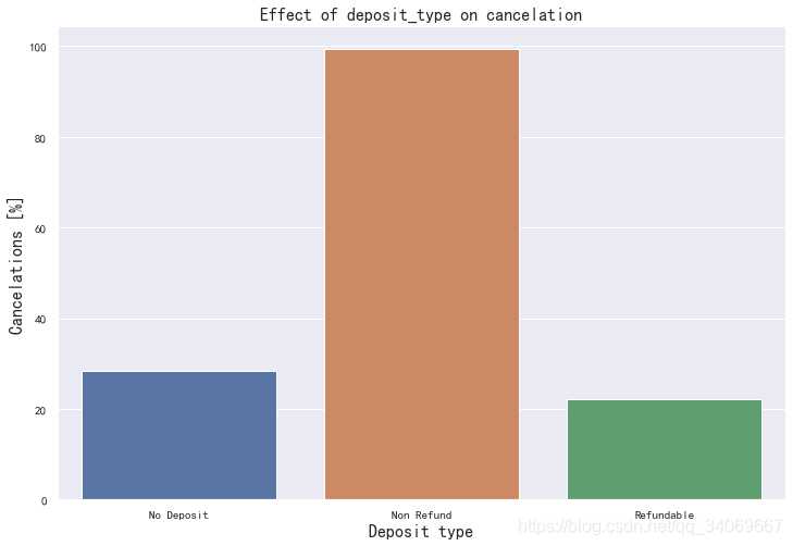
正如Susmit Vengurlekar在数据集的讨论部分已经指出的那样，存款类型“不退款”和“取消”列以一种反直觉的方式关联起来。

超过99%的预付款的人取消了。这就提出了一个问题：数据（或描述）是否有问题。

还有什么是不退款的存款？

以下是按存款类型分组的所有数据平均值表：

deposit_mean_data = data_new.groupby("deposit_type").mean()
deposit_mean_data

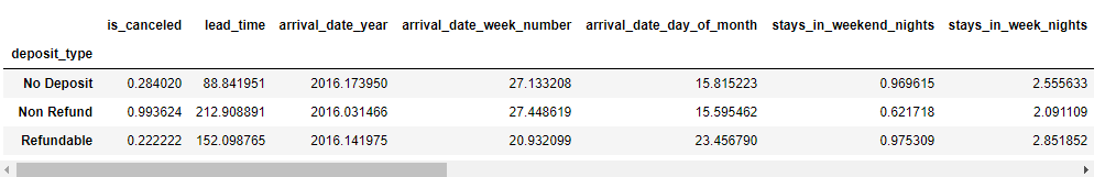
将不退款和不存款的平均值进行比较，结果如下：

• 不退还押金的特点是提前期延长2倍以上
• 重复的客人是~1/10
• 以前的取消次数是以前的10倍
• 以前的预订没有取消是1/15
• 所需的停车位几乎为零
• 特殊要求非常罕见

根据这些调查结果，似乎特别是那些没有预先参观过其中一家酒店的人，预订、付款并多次取消。。。真奇怪！
为了解决这个问题，接下来制作一个没有这个功能下面的模型。
ADR

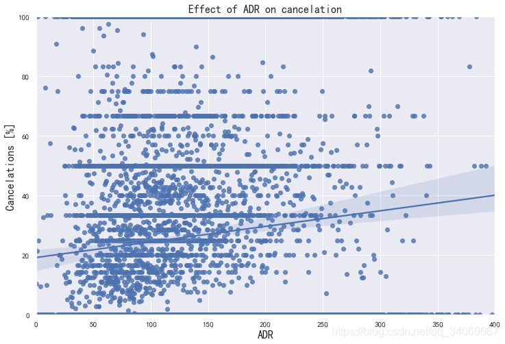
ADR越低取消的就越集中

RF model without deposit type

cat_features_non_dep = ["hotel","arrival_date_month","meal","market_segment",
                "distribution_channel","reserved_room_type","customer_type"]

features_non_dep = num_features + cat_features_non_dep
X_non_dep = data_new.drop(["is_canceled"], axis=1)[features_non_dep]


# Bundle preprocessing for numerical and categorical features:
preprocessor_non_dep = ColumnTransformer(transformers=[("num", num_transformer, num_features),
                                               ("cat", cat_transformer, cat_features_non_dep)])

# Define dataset:
X_non_dep = data_new.drop(["is_canceled"], axis=1)[features_non_dep]
# Define model
rf_model_non_dep = RandomForestClassifier(random_state=42) # basic model for this purpose

kfolds=4
split = KFold(n_splits=kfolds, shuffle=True, random_state=42)
model_pipe = Pipeline(steps=[('preprocessor', preprocessor_non_dep),
                              ('model', rf_model_non_dep)])
cv_results = cross_val_score(model_pipe, 
                                 X_non_dep, y, 
                                 cv=split,
                                 scoring="accuracy",
                                 n_jobs=-1)
# output:
min_score = round(min(cv_results), 4)
max_score = round(max(cv_results), 4)
mean_score = round(np.mean(cv_results), 4)
std_dev = round(np.std(cv_results), 4)
print(f"RF model without deposit_type feature cross validation accuarcy score: {mean_score} +/- {std_dev} (std) min: {min_score}, max: {max_score}")

结果：RF model without deposit_type feature cross validation accuarcy score: 0.8657 +/- 0.0003 (std) min: 0.8653, max: 0.8662

我们看到结果和之前的相差并不远，还是很有意义。
我们可以在新模型上增加前置时间、adr、特殊请求的总数量等来弥补这一点。

这个分析暂告一段落，当然后期可以针对模型进行优化和完善。

代码参考：https://www.kaggle.com/marcuswingen/eda-of-bookings-and-ml-to-predict-cancelations
不能上去的也可以在我的云盘下载代码：
链接：https://pan.baidu.com/s/1KXuJCKbGx5YrEx4XvFJWbA
提取码：713x