一、碎碎念
因为工作上有用到Excel做数据分析,之后慢慢接触到了Python做分析,做挖掘等。再然后就遇到了Kaggle这个网站,发现这里真是让人提升技能的圣地。一直在找些可以提升自己数据分析技能、思维的项目来练习,下面主要会展示一些自己的分析思路,可视化图表,以及代码。
我的分析环境是win7 64位 ,anaconda-spyder(Python3.6)
看了kaggle上这个项目各路大神的代码思路,然后自己也跃跃欲试要操刀一练。分析完这个项目,给自己的领悟是对于部分的语法,函数,有个进一步的理解,对于分析项目应该怎么一步步的分析也有了更新,在初识这个项目的时候是直接杠正面各种尝试,各种推理,毕竟一个人闭门造车有时候会造不出车。
写这篇文章也算是对这个项目的一个回顾和总结。
提醒一点,在kaggle上注册账号是可以的,但是要通过邮箱激活账户的时候需要一个VPN。(我用的163的邮箱)
二、项目背景
本文中用到的数据文件:tmdb_5000_movies.csv、tmdb_5000_credits.csv是Kaggle平台上的项目TMDB(The Movie Database),共计4803部电影,主要为美国地区一百年间(1916-2017)的电影作品。
本文通过对电影数据的分析,利用数据可视化的方法,发现流行趋势,找到投资方向,为本行业新入局者提供一定参考建议。同时也为了提升自己的数据分析能力,在遇到类似项目可以触类旁通。
三、项目概览
点击下图可以直接链接到Kaggle对应的项目:
 下面是官网内容简介:
Background
What can we say about the success of a movie before it is released? Are there certain companies (Pixar?) that have found a consistent formula? Given that major films costing over $100 million to produce can still flop, this question is more important than ever to the industry. Film aficionados might have different interests. Can we predict which films will be highly rated, whether or not they are a commercial success?
This is a great place to start digging in to those questions, with data on the plot, cast, crew, budget, and revenues of several thousand films.
We (Kaggle) have removed the original version of this dataset per a DMCA takedown request from IMDB. In order to minimize the impact, we're replacing it with a similar set of films and data fields from The Movie Database (TMDb) in accordance with their terms of use. The bad news is that kernels built on the old dataset will most likely no longer work.
The good news is that:
You can port your existing kernels over with a bit of editing. This kernel offers functions and examples for doing so. You can also find a general introduction to the new format here.
The new dataset contains full credits for both the cast and the crew, rather than just the first three actors.
Actor and actresses are now listed in the order they appear in the credits. It's unclear what ordering the original dataset used; for the movies I spot checked it didn't line up with either the credits order or IMDB's stars order.
The revenues appear to be more current. For example, IMDB's figures for Avatar seem to be from 2010 and understate the film's global revenues by over $2 billion.
Some of the movies that we weren't able to port over (a couple of hundred) were just bad entries. For example, this IMDB entry has basically no accurate information at all. It lists Star Wars Episode VII as a documentary.
Several of the new columns contain json. You can save a bit of time by porting the load data functions from this kernel.
Even in simple fields like runtime may not be consistent across versions. For example, previous dataset shows the duration for Avatar's extended cut while TMDB shows the time for the original version.
There's now a separate file containing the full credits for both the cast and crew.
All fields are filled out by users so don't expect them to agree on keywords, genres, ratings, or the like.
Your existing kernels will continue to render normally until they are re-run.
If you are curious about how this dataset was prepared, the code to access TMDb's API is posted here.
四、前置思路
“运筹帷幄,决胜千里。”古时候老司机的话对我们进行数据分析时依然有用。
我的习惯看到一个项目,先打开数据文件看看其中的数据是什么样子的,大概有多少字段,每个字段里的数据是个什么类型。
俗话说得好,让自己有点B数。
Kaggle平台上下载2个原始数据集:tmdb_5000_movies.csv和tmdb_5000_credits.csv,前者存放电影的基本信息,后者存放电影的演职员名单。
不管怎么样的数据分析任务都需要遵从一个标准流程,有了流程指导,分析思路和处理过程才不会让自己进入迷失森林。
数据分析的流程:1.提出问题2.理解数据3.数据清洗4.建立模型5.数据可视化6.形成数据分析报告
五、提出问题
如果我是电影行业的数据分析师,一定要让自己身临其境站在制作公司的角度出发去思考。(这一点很关键)
现在公司要制作电影,想知道电影预算、评分与票房的关系,各种电影类型随时间变化的趋势图,电影产量、票房的趋势,哪些风格电影最受欢迎等问题,则可提出如下问题:
问题1:电影风格随时间的变化趋势
问题2:不同风格电影的收益能力
问题3:比较行业内Universal Pictures与Paramount Pictures两家巨头公司的业绩
问题4:票房收入与哪些因素最相关
六、理解数据
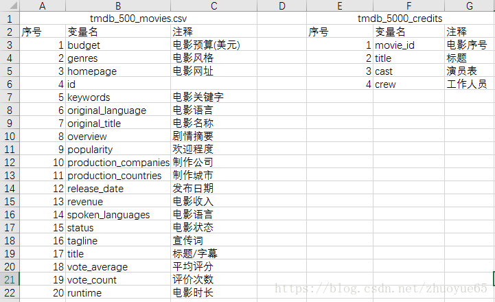
下面的变量名是数据中出现的,也是2个数据表格中的列名。
七、数据清洗
数据清洗主要分三步:1.数据预处理;2.特征提取;3.特征选取。
7.1 数据预处理
在数据预处理时,主要包括:发现和填补缺失值、数据类型转换、异常值删除等。数据中release_date列缺失1条数据,runtime列缺失2条数据,均可通过索引的方式找到具体是哪一部电影,然后上网搜索准确的缺失数据,将其填补(详见后续代码)。对于release_date列,需将其转换为日期类型,然后提取出“年份”数据。
7.2 特征提取
在我们处理数据的过程中:通过json.loads先将JSON字符串转换为字典列表"[{},{},{}]"的形式,再遍历每个字典,取出键(key)为‘name’所对应的值(value),并将这些值(value)用“|”分隔,形成一个“多选题”的结构。在进行具体问题分析的时候,再将“多选题”编码为虚拟变量,即所有多选题的每一个不重复的选项,拿出来作为新变量,每一条观测包含该选项则填1,否则填0。
7.3 特征选取
在分析每一个小问题之前,最重要的步骤是需要通过特征选取,构造出适合分析的结构,只有结构“造”对了,后续的可视化才能得出正确的图形。
这里的小窍门就是:分析每一个小问题时,尽量新建一个数据框,存放要分析的变量,而不是在原始数据框上“乱涂乱画”,否则最后必定抓狂。
八、数据可视化
本次使用到的图形类型有:柱状图、饼图、散点图。
九、代码部分
首先我们需要代入一些用到的包,并不是一下子就要导入pandas、numpy、matplotlib等等,包是在写代码的时候遇到问题一个个添加的,然后写到最前面。
9.1理解数据
import numpy as np
import pandas as pd
import matplotlib.pyplot as plt
import matplotlib
#%matplotlib inline
import json
import warnings
warnings.filterwarnings('ignore')

import seaborn as sns
sns.set(color_codes=True)

#设置表格用什么字体
font = {
    'family' : 'SimHei'
}
matplotlib.rc('font', **font)

#导入数据
movies = pd.read_csv('C:\\kaggle_from0\\tmdb_5000_movies\\tmdb_5000_movies.csv')
creditss = pd.read_csv('C:\\kaggle_from0\\tmdb_5000_movies\\tmdb_5000_credits.csv')

#查看movies中数据
movies.head()

#查看movies中所有列名,以字典形式存储
movies.columns

##查看creditss中数据
creditss.head()

#查看creditss中所有列名,以字典形式存储,一共4个列名
creditss.columns

#两个数据框中的title列重复了,删除credits中的title列,还剩3个列名
del creditss['title']

#movies中的id列与credits中的movie_id列实际上等同,可当做主键合并数据框
full = pd.merge(movies, creditss, left_on='id', right_on='movie_id', how='left')

#某些列不在本次研究范围,将其删除
full.drop(['homepage','original_title','overview','spoken_languages',
           'status','tagline','movie_id'],axis=1,inplace=True)

#查看数据信息,每个字段数据量。
full.info()
9.2数据清洗
首先,判断哪些列有缺失值,以Ture=缺失, False=不缺失,得到release_date,runtime有缺失值。
full.isnull().any()
release_date列有1条缺失数据,将其查找出来
full.loc[full['release_date'].isnull()==True]
根据title经上网搜索,该影片上映日期为2014年6月1日,填补该值
full['release_date'] = full['release_date'].fillna('2014-06-01')
runtime列有2条缺失数据,将其查找出来
full.loc[full['runtime'].isnull()==True]
根据title经上网搜索,影片时长分别为94分钟和240分钟,填补缺失值
full['runtime'] = full['runtime'].fillna(94, limit=1)#limit=1,限制每次只填补一个值
full['runtime'] = full['runtime'].fillna(240, limit=1)
将release_date列转换为日期类型
full['release_date'] = pd.to_datetime(full['release_date'],
    format='%Y-%m-%d', errors='coerce').dt.year
genres,keywords,production_companies,production_countries,cast,crew列为json类型
需要解析json数据,分两步:
1. json本身为字符串类型,先转换为字典列表
2. 再将字典列表转换为,以'|'分割的字符串
定义一个json类型的列名列表
json_column = ['genres','keywords','production_companies',
               'production_countries','cast','crew']
将各json列转换为字典列表
for column in json_column:
    full[column]=full[column].map(json.loads)
函数功能:将字典内的键‘name’对应的值取出,生成用'|'分隔的字符串
def getname(x):
    list = []
    for i in x:
        list.append(i['name'])
    return '|'.join(list)
对genres,keywords,production_companies,production_countries列执行函数
for column in json_column[0:4]:
    full[column] = full[column].map(getname)
定义提取2名主演的函数:
def getcharacter(x):
    list = []
    for i in x:
        list.append(i['character'])
    return '|'.join(list[0:2])
对cast列执行函数
full['cast']=full['cast'].map(getcharacter)
定义提取导演的函数:
def getdirector(x):
    list=[]
    for i in x:
        if i['job']=='Director':
            list.append(i['name'])
    return "|".join(list)
对crew列执行函数
full['crew']=full['crew'].map(getdirector)
重命名列
rename_dict = {'release_date':'year','cast':'actor','crew':'director'}
full.rename(columns=rename_dict, inplace=True)
查看full表格中前2行数据
full.head(2)
备份原始数据框original_df
original_df = full.copy()
到此为止,我们的数据预处理告一段落。
9.3数据可视化
9.3.1问题1:研究电影风格随时间的变化趋势,提取所有的电影风格,存储在有去重功能的集合中。
genre_set = set()   #设置空集合
for x in full['genres']:
    genre_set.update(x.split('|'))  #genres数据以'|'来分隔
genre_set.discard('')  #删除''字符
对各种电影风格genre,进行one-hot编码
genre_df = pd.DataFrame()  # 创建空的数据框
for genre in genre_set:
    #如果一个值中包含特定内容,则编码为1,否则编码为0
    genre_df[genre] = full['genres'].str.contains(genre).map(lambda x:1 if x else 0)
将原数据集中的year列,添加至genre_df数据框中
genre_df['year']=full['year']
将genre_df按year分组,计算每组之和。groupby之后,year列通过默认参数as_index=True自动转化为df.index
genre_by_year = genre_df.groupby('year').sum()
genresum_by_year = genre_by_year.sum().sort_values(ascending=False)
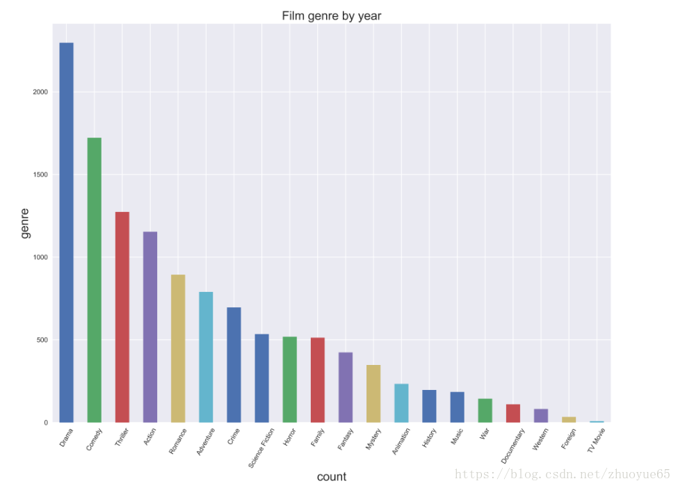
计算每个风格genre的电影总数目,并降序排列,再可视化
fig = plt.figure(figsize=(15,11))   #设置画图框的大小
ax = plt.subplot(1,1,1)     #设置框的位置
ax = genresum_by_year.plot.bar()
plt.xticks(rotation=60)
plt.title('Film genre by year', fontsize=18)    #设置标题的字体大小,标题名
plt.xlabel('count', fontsize=18)    #X轴名及轴名大小
plt.ylabel('genre', fontsize=18)    #y轴名及轴名大小
plt.show()  #可以用查看数据画的图。
#保存图片
fig.savefig('film genre by year.png',dpi=600)
筛选出电影风格TOP8
genre_by_year = genre_by_year[['Drama','Comedy','Thriller','Romance',
                               'Adventure','Crime', 'Science Fiction',
                               'Horror']].loc[1960:,:]
year_min = full['year'].min()   #最小年份
year_max = full['year'].max()   #最大年份
可视化电影风格genre随时间的变化趋势(1960年至今)
fig = plt.figure(figsize=(10,8))
ax1 = plt.subplot(1,1,1)
plt.plot(genre_by_year)
plt.xlabel('Year', fontsize=12)
plt.ylabel('Film count', fontsize=12)
plt.title('Film count by year', fontsize=15)
plt.xticks(range(1960, 2017, 10))  #横坐标每隔10年一个刻度
#plt.legend(loc='best',ncol=2) #https://blog.csdn.net/you_are_my_dream/article/details/53440964
plt.legend(['Drama(戏剧类)','Comedy(喜剧类)','Thriller(惊悚类)','Romance(浪漫类)',
                               'Adventure(Adventure)','Crime(犯罪类)', 'Science Fiction(科幻类)',
                               'Horror(惊恐类)'], loc='best',ncol=2) #设置说明标签
fig.savefig('film count by year.png',dpi=200)
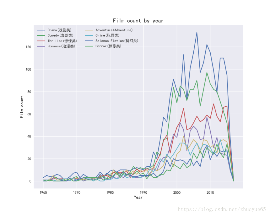
可以看出,从上世纪90年代开始,整个电影市场呈现爆发式增长。其中,排名前五的戏剧类(Drama)、喜剧类(Comedy)、惊悚类(Thriller)、浪漫类(Romance)、冒险类(Adventure)电影数量增长显著。
9.3.2问题2:不同风格电影的收益能力
增加收益列
full['profit'] = full['revenue']-full['budget']
创建收益数据框
profit_df = pd.DataFrame()#创建空的数据框
profit_df = pd.concat([genre_df.iloc[:,:-1],full['profit']],axis=1)  #合并
profit_df.head()#查看新数据框信息
创建一个Series,其index为各个genre,值为按genre分类计算的profit之和
profit_by_genre = pd.Series(index=genre_set)
for genre in genre_set:
    profit_by_genre.loc[genre]=profit_df.loc[:,[genre,'profit']].groupby(genre, as_index=False).sum().loc[1,'profit']
print(profit_by_genre)
创建一个Series,其index为各个genre,值为按genre分类计算的budget之和
budget_df = pd.concat([genre_df.iloc[:,:-1],full['budget']],axis=1)
budget_df.head(2)
budget_by_genre = pd.Series(index=genre_set)
for genre in genre_set:
    budget_by_genre.loc[genre]=budget_df.loc[:,[genre,'budget']].groupby(genre,as_index=False).sum().loc[1,'budget']
print(budget_by_genre)
向合并数据框
profit_rate = pd.concat([profit_by_genre, budget_by_genre],axis=1)
profit_rate.columns=['profit','budget']   #更改列名
加收益率列
profit_rate['profit_rate'] = (profit_rate['profit']/profit_rate['budget'])*100
profit_rate.sort_values(by=['profit','profit_rate'], ascending=False, inplace=True)
#print(profit_rate)
x为索引长度的序列
x = list(range(len(profit_rate.index)))
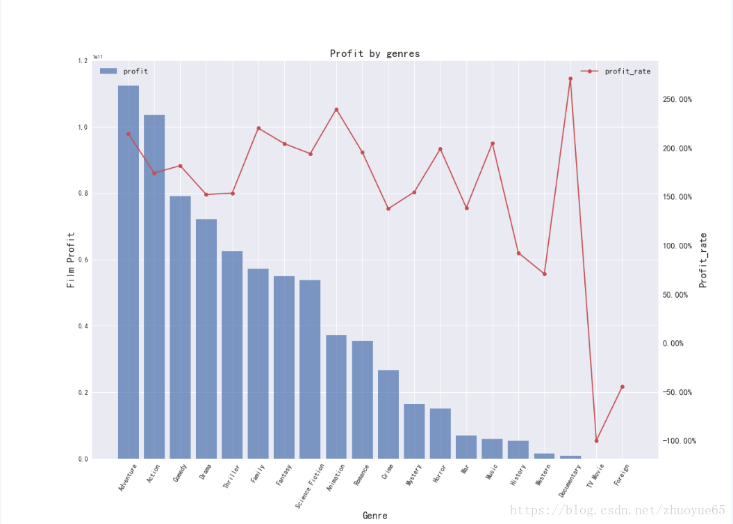
可视化不同风格电影的收益(柱状图)和收益率(折线图)
fig = plt.figure(figsize=(18,13))
ax1 = fig.add_subplot(111)
plt.bar(x, profit_rate['profit'],label='profit',alpha=0.7)
plt.xticks(x,xl,rotation=60,fontsize=12)
plt.yticks(fontsize=12)
ax1.set_title('Profit by genres', fontsize=20)
ax1.set_ylabel('Film Profit',fontsize=18)
ax1.set_xlabel('Genre',fontsize=18)
ax1.set_ylim(0,1.2e11)
ax1.legend(loc=2,fontsize=15)
次纵坐标轴标签设置为百分比显示
import matplotlib.ticker as mtick
ax2 = ax1.twinx()
ax2.plot(x, profit_rate['profit_rate'],'ro-',lw=2,label='profit_rate')
fmt='%.2f%%'
yticks = mtick.FormatStrFormatter(fmt)
ax2.yaxis.set_major_formatter(yticks)
plt.xticks(x,xl,fontsize=12,rotation=60)
plt.yticks(fontsize=15)
ax2.set_ylabel('Profit_rate',fontsize=18)
ax2.legend(loc=1,fontsize=15)
plt.grid(False)
#保存图片
fig.savefig('profit by genres.png')
9.3.3问题3:比较Universal Pictures与Paramount Pictures两家巨头公司的业绩
创建公司数据框
company_list = ['Universal Pictures', 'Paramount Pictures']
company_df = pd.DataFrame()
for company in company_list:
    company_df[company]=full['production_companies'].str.contains(company).map(lambda x:1 if x else 0)
company_df = pd.concat([company_df,genre_df.iloc[:,:-1],full['revenue']],axis=1)
创建巨头对比数据框
Uni_vs_Para = pd.DataFrame(index=['Universal Pictures', 'Paramount Pictures'],
                           columns=company_df.columns[2:])
计算两家公司各自收益总额
Uni_vs_Para.loc['Universal Pictures']=company_df.groupby('Universal Pictures',
               as_index=False).sum().iloc[1,2:]
Uni_vs_Para.loc['Paramount Pictures']=company_df.groupby('Paramount Pictures',
               as_index=False).sum().iloc[1,2:]
可视化两公司票房收入对比
fig = plt.figure(figsize=(4,3))
ax = fig.add_subplot(111)
Uni_vs_Para['revenue'].plot(ax=ax,kind='bar')
plt.xticks(rotation=0)
plt.title('Universal VS. Paramount')
plt.ylabel('Revenue')
fig.savefig('Universal vs Paramount by revenue.png')
"""Universal Pictrues总票房收入高于Paramount Pictures"""
Uni_vs_Para = Uni_vs_Para.T
分解两公司数据框
universal = Uni_vs_Para['Universal Pictures'].iloc[:-1]
paramount = Uni_vs_Para['Paramount Pictures'].iloc[:-1]
将universal数量排名9之后的加和,命名为others
universal['others']=universal.sort_values(ascending=False).iloc[8:].sum()
universal = universal.sort_values(ascending=True).iloc[-9:]
将paramount数量排名9之后的加和,命名为others
paramount['others']=paramount.sort_values(ascending=False).iloc[8:].sum()
paramount = paramount.sort_values(ascending=True).iloc[-9:]
可视化两公司电影风格数量占比
fig = plt.figure(figsize=(13,6))
ax1 = plt.subplot(1,2,1)
ax1 = plt.pie(universal, labels=universal.index, autopct='%.2f%%',startangle=90,pctdistance=0.75)
plt.title('Universal Pictures',fontsize=15)

ax2 = plt.subplot(1,2,2)
ax2 = plt.pie(paramount, labels=paramount.index, autopct='%.2f%%',startangle=90,pctdistance=0.75)
plt.title('Paramount Pictures',fontsize=15)
9.3.4问题4:看看票房与哪些因素有关
full[['runtime','popularity','vote_average',
      'vote_count','budget','revenue']].corr()
受欢迎度和票房相关性:0.64评价次数和票房相关性:0.78
电影预算和票房相关性:0.73
创建票房收入数据框
revenue = full[['popularity','vote_count','budget','revenue']]
可视化票房收入分别与受欢迎度(蓝)、评价次数(绿)、电影预算(红)的相关性散点图,并配线性回归线。
fig = plt.figure(figsize=(17,5))
ax1 = plt.subplot(1,3,1)
ax1 = sns.regplot(x='popularity', y='revenue', data=revenue, x_jitter=.1)
ax1.text(400,2e9,'r=0.64',fontsize=15)
plt.title('revenue by popularity',fontsize=15)
plt.xlabel('popularity',fontsize=13)
plt.ylabel('revenue',fontsize=13)

ax2 = plt.subplot(1,3,2)
ax2 = sns.regplot(x='vote_count', y='revenue', data=revenue, x_jitter=.1,color='g',marker='+')
ax2.text(6800,1.1e9,'r=0.78',fontsize=15)
plt.title('revenue by vote_count',fontsize=15)
plt.xlabel('vote_count',fontsize=13)
plt.ylabel('revenue',fontsize=13)

ax3 = plt.subplot(1,3,3)
ax3 = sns.regplot(x='budget', y='revenue', data=revenue, x_jitter=.1,color='r',marker='^')
ax3.text(1.6e8,2.2e9,'r=0.73',fontsize=15)
plt.title('revenue by budget',fontsize=15)
plt.xlabel('budget',fontsize=13)
plt.ylabel('revenue',fontsize=13)
fig.savefig('revenue.png')
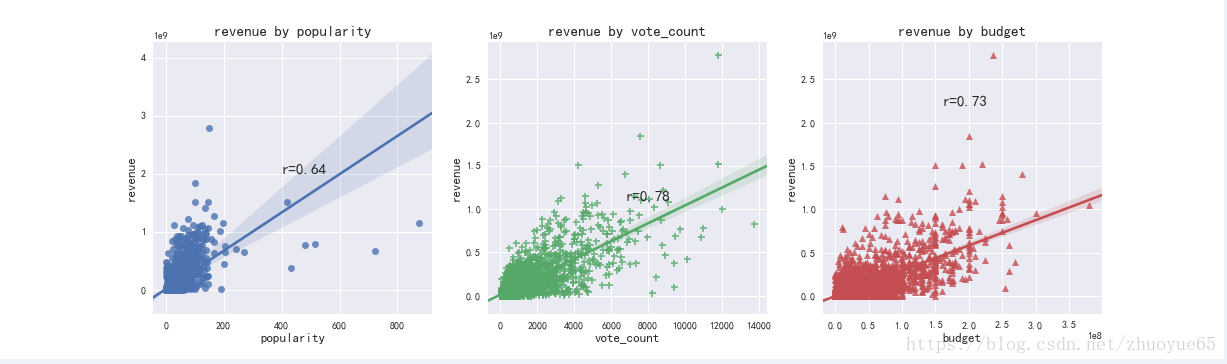
电影评次与票房收入最相关(绿色),电影预算与票房收入高度相关(红色),受欢迎度与评次高度相关,因此与票房收入相关性较高。
建议:增加电影预算 用于电影本身、多用于渠道宣传
十、一些分析中用到的语法,当时查阅了资料整理一下。
(下次补充)