MXNET深度学习框架-18-使用gluon实现VGGNet

      VGGNet与上一章的AlexNet相比，模型更深，非线性表达能力更强，原因在于它将一系列 $7×7$、 $5×5$的卷积核变成了几个反复堆叠的 $3×3$卷积，比如：2个 $3×3$的卷积可以替代 $7×7$的卷积、3个 $3×3$的卷积可以替代 $5×5$的卷积。这样做不仅不会增加参数量，反而会增加模型的非线性表达能力。

      下面使用mxnet实现VGGNet：

1、VGG Block实现：
      比如我有一100个卷积层（当然VGG不可能成功，因为会发生梯度消失等现象），难道说我要写1000行代码？所以需要定义一个Block，反正VGG全部用的是 $3×3$的卷积。

def VGG_Block(num_convs,channels):
    net=gn.nn.Sequential()
    with net.name_scope():
        for i in range(num_convs):
            net.add(gn.nn.Conv2D(channels=channels,kernel_size=3,padding=1,
                                 activation="relu"))
        net.add(gn.nn.MaxPool2D(pool_size=(2,2),strides=2))
    return net

接下来实例化一个例子看看：

X=nd.random.normal(shape=(2,3,16,16))
blk=VGG_Block(2,128) # 2个堆叠的3X3卷积，相当于5X5
blk.initialize()
y=blk(X)
print(y.shape)

运行结果：

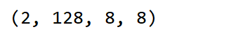
原维度是3，经过VGG Block之后，特征维度变成了128，由于使用了最大池化，所以大小由(16,16)变成了(8,8)。为什么要这么做？长宽减小，深就要增加，这样能保持基本的信息不变。

2、VGG-11实现
      包含8个卷积层、3个全连接：

# 它有5个卷积块，前2块使用单卷积层，而后3块使用双卷积层。
# 第一块的输出通道是64，之后每次对输出通道数翻倍，直到变为512。
# 因为这个网络使用了8个卷积层和3个全连接层，所以经常被称为VGG-11。
architecture=((1,64),(1,128),(2,256),(2,512),(2,512))
def vgg(architecture):
    net=gn.nn.Sequential()
    with net.name_scope():
        for (num_conv,num_feature) in architecture:
            net.add(VGG_Block(num_conv,num_feature))
        # 全连接
        net.add(gn.nn.Flatten())
        net.add(gn.nn.Dense(4096,activation="relu"))
        net.add(gn.nn.Dropout(0.5))
        net.add(gn.nn.Dense(4096, activation="relu"))
        net.add(gn.nn.Dropout(0.5))
        net.add(gn.nn.Dense(10))
    return net

我们运行一个实例看看维度：

net=vgg(architecture)
net.initialize()
X = nd.random.uniform(shape=(1, 1, 224, 224))
for blk in net:
    X = blk(X)
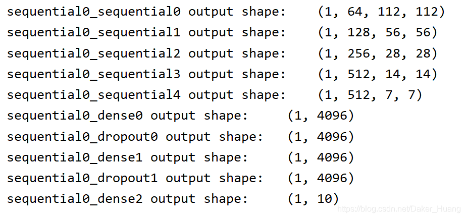
    print(blk.name, 'output shape:\t', X.shape)

结果：

为了便于训练，我把全连接层的参数改小，图片输入大小也改小了，下面附上所有代码：

import mxnet.gluon as gn
import mxnet.autograd as ag
import mxnet.ndarray as nd
import mxnet.initializer as init
import mxnet as mx

# 反复堆叠的conv
def VGG_Block(num_convs,channels):
    net=gn.nn.Sequential()
    with net.name_scope():
        for i in range(num_convs):
            net.add(gn.nn.Conv2D(channels=channels,kernel_size=3,padding=1,
                                 activation="relu"))
        net.add(gn.nn.MaxPool2D(pool_size=(2,2),strides=2))
    return net
# 实例化一个例子看看
# X=nd.random.normal(shape=(2,3,16,16))
# blk=VGG_Block(2,128) # 2个堆叠的3X3卷积，相当于5X5
# blk.initialize()
# y=blk(X)
# print(y.shape)
# 现在我们构造一个VGG网络。
# 它有5个卷积块，前2块使用单卷积层，而后3块使用双卷积层。
# 第一块的输出通道是64，之后每次对输出通道数翻倍，直到变为512。
# 因为这个网络使用了8个卷积层和3个全连接层，所以经常被称为VGG-11。
ctx=mx.gpu()
architecture=((1,64),(1,128),(2,256),(2,512),(2,512))
def vgg(architecture):
    net=gn.nn.Sequential()
    with net.name_scope():
        for (num_conv,num_feature) in architecture:
            net.add(VGG_Block(num_conv,num_feature))
        # 全连接
        net.add(gn.nn.Flatten())
        net.add(gn.nn.Dense(256,activation="relu"))  # VGG的全连接层神经元太大，为便于训练改小一点
        net.add(gn.nn.Dropout(0.5))
        net.add(gn.nn.Dense(128, activation="relu"))
        net.add(gn.nn.Dropout(0.5))
        net.add(gn.nn.Dense(10))
    return net
net=vgg(architecture)
net.initialize(ctx=ctx,init=init.Xavier())
# print(net)
# X = nd.random.uniform(shape=(1, 1, 28, 28))
# for blk in net:
#     X = blk(X)
#     print(blk.name, 'output shape:\t', X.shape)

'''---读取数据和预处理---'''
def load_data_fashion_mnist(batch_size, resize=None):
    transformer = []
    if resize:
        transformer += [gn.data.vision.transforms.Resize(resize)]
    transformer += [gn.data.vision.transforms.ToTensor()]
    transformer = gn.data.vision.transforms.Compose(transformer)
    mnist_train = gn.data.vision.FashionMNIST(train=True)
    mnist_test = gn.data.vision.FashionMNIST(train=False)
    train_iter = gn.data.DataLoader(
        mnist_train.transform_first(transformer), batch_size, shuffle=True)
    test_iter = gn.data.DataLoader(
        mnist_test.transform_first(transformer), batch_size, shuffle=False)
    return train_iter, test_iter
batch_size=64
train_iter,test_iter=load_data_fashion_mnist(batch_size,resize=32) # 32,因为图片加大的话训练很慢，而且显存会吃不消
# softmax和交叉熵损失函数
# 由于将它们分开会导致数值不稳定(前两章博文的结果可以对比)，所以直接使用gluon提供的API
cross_loss=gn.loss.SoftmaxCrossEntropyLoss()

# 定义准确率
def accuracy(output,label):
    return nd.mean(output.argmax(axis=1)==label).asscalar()

def evaluate_accuracy(data_iter,net):# 定义测试集准确率
    acc=0
    for data,label in data_iter:
        data, label = data.as_in_context(ctx), label.as_in_context(ctx)
        label = label.astype('float32')
        output=net(data)
        acc+=accuracy(output,label)
    return acc/len(data_iter)

# softmax和交叉熵分开的话数值可能会不稳定
cross_loss=gn.loss.SoftmaxCrossEntropyLoss()
# 优化
train_step=gn.Trainer(net.collect_params(),'sgd',{"learning_rate":0.01})

# 训练
lr=0.1
epochs=20
for epoch in range(epochs):
    n=0
    train_loss=0
    train_acc=0
    for image,y in train_iter:
        image, y = image.as_in_context(ctx), y.as_in_context(ctx)
        y = y.astype('float32')
        with ag.record():
            output = net(image)
            loss = cross_loss(output, y)
        loss.backward()
        train_step.step(batch_size)
        train_loss += nd.mean(loss).asscalar()
        train_acc += accuracy(output, y)

    test_acc = evaluate_accuracy(test_iter, net)
    print("Epoch %d, Loss:%f, Train acc:%f, Test acc:%f"
          %(epoch,train_loss/len(train_iter),train_acc/len(train_iter),test_acc))

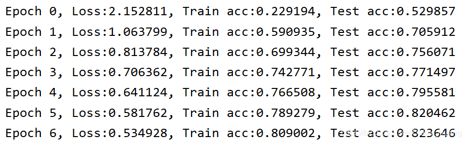
训练结果：