原文链接:http://tecdat.cn/?p=12187
金融分析师通常关心检测市场何时“发生变化”:几个月或至几年内市场的典型行为可以立即转变为非常不同的行为。投资者希望及时发现这些变化,以便可以相应地调整其策略,但是这样做可能很困难。
RHmm从CRAN不再可用,因此我想使用其他软件包复制功能实现马尔科夫机制转换(Markov regime switching)模型从而对典型的市场行为进行预测,并且增加模型中对参数的线性约束功能。
library(SIT)
load.packages('quantmod')

	# find regimes
	load.packages('RHmm', repos ='http://R-Forge.R-project.org')

	y=returns
	ResFit = HMMFit(y, nStates=2)
	VitPath = viterbi(ResFit, y)
DimObs = 1
	matplot(fb$Gamma, type='l', main='Smoothed Probabilities', ylab='Probability')
		legend(x='topright', c('State1','State2'),  fill=1:2, bty='n')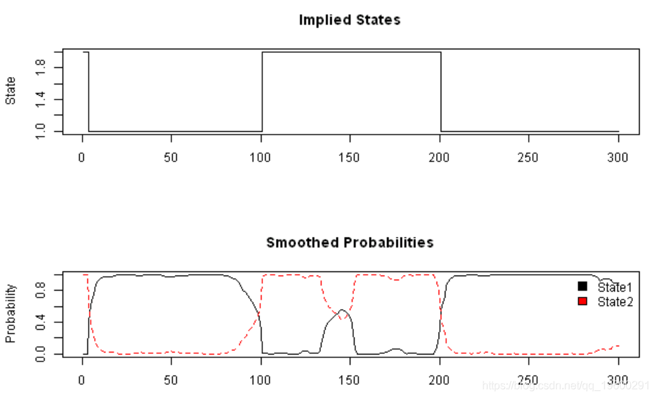
![]()
fm2 = fit(mod, verbose = FALSE)使用logLik在迭代69处收敛:125.6168
	probs = posterior(fm2)

	layout(1:2)
	plot(probs$state, type='s', main='Implied States', xlab='', ylab='State')

	matplot(probs[,-1], type='l', main='Probabilities', ylab='Probability')
		legend(x='topright', c('State1','State2'),  fill=1:2, bty='n')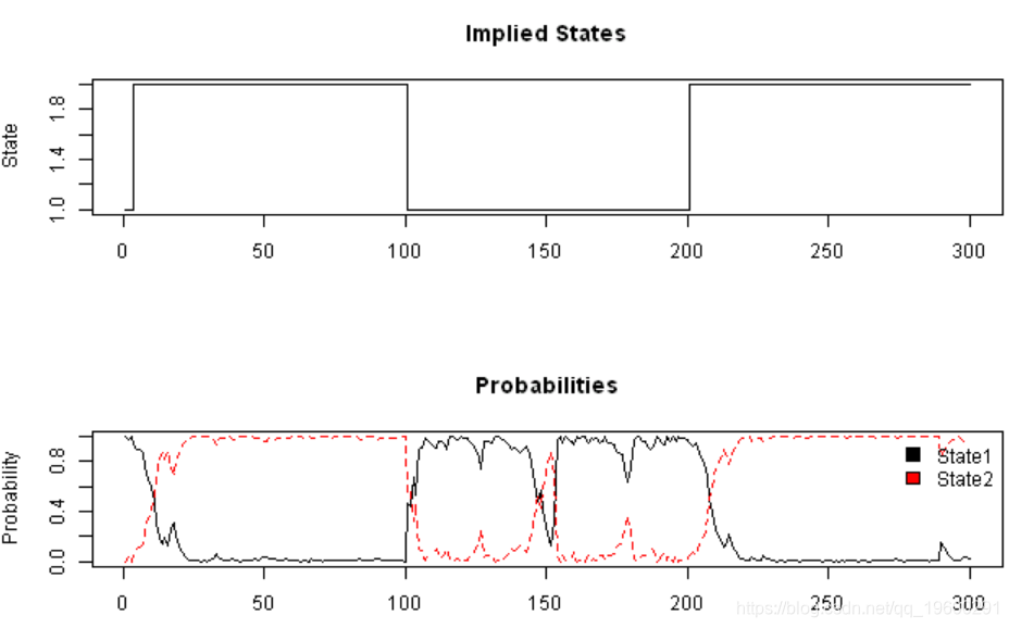
![]()
	#*****************************************************************
	# Add some data and see if the model is able to identify the regimes
	#******************************************************************
	bear2  = rnorm( 100, -0.01, 0.20 )
	bull3 = rnorm( 100, 0.10, 0.10 )
	bear3  = rnorm( 100, -0.01, 0.25 )
	true.states = c(true.states, rep(2,100),rep(1,100),rep(2,100))
	y = c( bull1, bear,  bull2, bear2, bull3, bear3 )
DimObs = 1
	plota(data, type='h', x.highlight=T)
		plota.legend('Returns + Detected Regimes')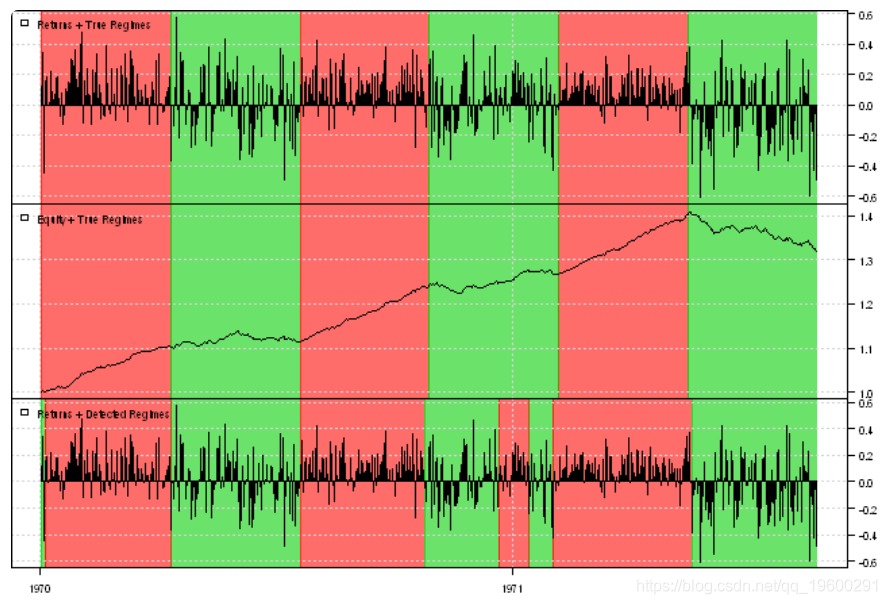
![]()
#*****************************************************************
# Load historical prices
#******************************************************************
data = env()
getSymbols('SPY', src = 'yahoo', from = '1970-01-01', env = data, auto.assign = T)

price = Cl(data$SPY)
	open = Op(data$SPY)
ret = diff(log(price))
	ret = log(price) - log(open)

atr = ATR(HLC(data$SPY))[,'atr']

fm2 = fit(mod, verbose = FALSE)
使用logLik在迭代30处收敛:18358.98
print(summary(fm2))Initial state probabilties model pr1 pr2 pr3 pr4 0 0 1 0
Transition matrix toS1 toS2 toS3 toS4 fromS1 9.821940e-01 1.629595e-02 1.510069e-03 8.514403e-45 fromS2 1.167011e-02 9.790209e-01 8.775478e-68 9.308946e-03 fromS3 3.266616e-03 8.586650e-47 9.967334e-01 1.350529e-69 fromS4 3.608394e-65 1.047516e-02 1.922545e-130 9.895248e-01
Response parameters Resp 1 : gaussian Resp 2 : gaussian Re1.(Intercept) Re1.sd Re2.(Intercept) Re2.sd St1 2.897594e-04 0.006285514 1.1647547 0.1181514 St2 -6.980187e-05 0.008186433 1.6554049 0.1871963 St3 2.134584e-04 0.005694483 0.4537498 0.1564576 St4 -4.459161e-04 0.015419207 2.7558362 0.7297283
Re1.(Intercept) Re1.sd Re2.(Intercept) Re2.sd
St1 0.000289759401378951 0.00628551404616354 1.16475474419891 0.118151350440916
St2 -6.98018749098021e-05 0.00818643307634358 1.65540488736983 0.187196307284941
St3 0.000213458358141314 0.00569448330115608 0.453749781945066 0.156457606460757
St4 -0.00044591612667264 0.0154192070819596 2.75583620018895 0.72972830143278
probs = posterior(fm2)

print(head(probs))
rownames(x) state S1 S2 S3 S4
1 3 0 0 1 0
2 3 0 0 1 0
3 3 0 0 1 0
4 3 0 0 1 0
5 3 0 0 1 0
6 3 0 0 1 0layout(1:3)
plota(temp, type='l', col='darkred')
plota.legend('Market Regimes', 'darkred')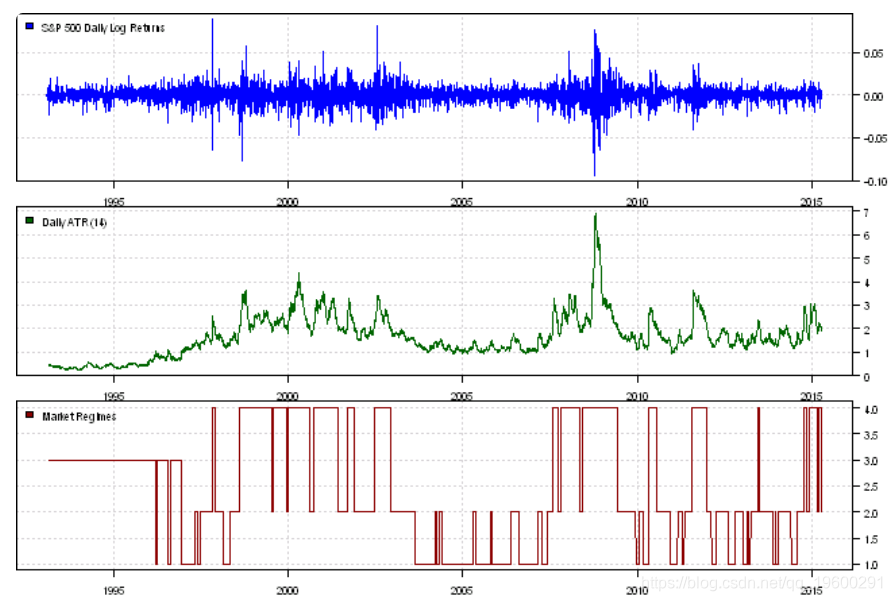
![]()
layout(1:4)
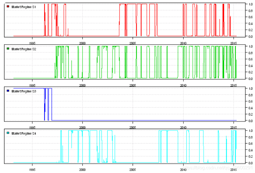
![]()