当天空一只鸟飞过去的时候,往往注意力会追随者鸟儿,天空在视觉系统中,自然成为了一个背景信息。

计算机视觉中的注意力机制(attention)的基本思想就是想让系统学会注意力——能够忽略无关信息而关注重点信息。在深度学习发展的今天,搭建能够具备注意力机制的神经网络则开始显得更加重要,一方面是这种神经网络能够自主学习注意力机制,另一方面是注意力机制能够反过来帮助我们去理解神经网络看到的世界。近几年来,深度学习与视觉注意力机制结合的研究工作,大多数是集中于使用掩码(mask)来形成注意力机制。掩码的原理在于通过另一层新的权重,将图片数据中关键的特征标识出来,通过学习训练,让深度学习网络学到每一张新图片中需要关注的区域,也就是形成了注意力。这种思想,进而演化成两种不同类型的注意力,一种是软注意力机制,另一种是强注意力机制。软注意力的关键点在于,这种注意力更加关注区域或者通道,而且软注意力是确定性注意力,学习完成后直接可以通过网络生成,最关键的地方是软注意力是可微的。强注意力更关注点,也就是图像中的每个点都有可能延申出注意力,同时强注意力是一个随机的预测过程,更强调动态变化,当然,最关键的是强注意力是一个不可微的注意力。注意力域主要有三种:空间域(spatial domain),通道域(channel domain),混合域(mixed domain)。
1.软注意力的注意力域 (soft attention)
1.1 空间域(Spatial domain)
设计思路:通过注意力机制,将原始图片的空间信息变换到另一个空间中并保留了关键信息。因为卷积神经网络中的池化层直接用最大池化或者平均池化的方法,将图片信息压缩,减少运算量提升准确率。但是这样的池化方法太过于暴力,直接将信息合并会导致关键信息无法识别出来,所以提出了一个叫空间转换器(spatial transformer)的模块,将图片中的空间域信息做对应的空间变换,从而将关键信息提取出来。

比如这个直观的实验图:a列是原始图片信息,其中第一个手写数字7没有做任何变换,第二个手写数字5,做了一定的旋转变化,而第三个手写数字6,加上了一些噪声信号;b列中的彩色边框是学习到的spatial transformer的框盒(bounding box),每一个框盒其实就是对应图片学习出来的一个spatial transformer;c列中是通过spatial transformer转换之后的特征图,可以看出7的关键区域被选择出来,5被旋转成为了正向的图片,6的噪声信息没有被识别进入。最终可以通过这些转换后的特征图来预测出d列中手写数字的数值。
spatial transformer其实就是注意力机制的实现,因为训练的空间转换器能够找出图片信息中需要被关注的区域,同时这个转换器又能够具有旋转、缩放变换的功能,这样图片的局部重要信息能够通过变换而被框盒提取出来。
模型结构如下:

这是空间变换网络(spatial transformer network)中最重要的空间变换模块,这个模块可以作为新的层直接加入到原有的网络结构,比如ResNet中。来仔细研究这个模型的输入:![]() 。神经网络训练中使用的数据类型都是张量(tensor),H是上一层tensor的高度(height),W是上一层tensor的宽度(width),而C代表tensor的通道(channel),比如图片基本的三通道(RGB),或者是经过卷积层(convolutional layer)之后,不同卷积核(kernel)都会产生不同的通道信息。之后这个输入进入两条路线,一条路线是信息进入定位网络(localisation net),另一条路线是原始信号直接进入采样层(sampler)。其中定位网络会学习到一组参数θ,而这组参数就能够作为网格生成器(grid generator)的参数,生成一个采样信号,这个采样信号其实是一个变换矩阵Tθ(G),与原始图片相乘之后,可以得到变换之后的矩阵V。
。神经网络训练中使用的数据类型都是张量(tensor),H是上一层tensor的高度(height),W是上一层tensor的宽度(width),而C代表tensor的通道(channel),比如图片基本的三通道(RGB),或者是经过卷积层(convolutional layer)之后,不同卷积核(kernel)都会产生不同的通道信息。之后这个输入进入两条路线,一条路线是信息进入定位网络(localisation net),另一条路线是原始信号直接进入采样层(sampler)。其中定位网络会学习到一组参数θ,而这组参数就能够作为网格生成器(grid generator)的参数,生成一个采样信号,这个采样信号其实是一个变换矩阵Tθ(G),与原始图片相乘之后,可以得到变换之后的矩阵V。![]()

通过这张转换图片,可以看出空间转换器中产生的采样矩阵是能够将原图中关键的信号提取出来,(a)中的采样矩阵是单位矩阵,不做任何变换,(b)中的矩阵是可以产生缩放旋转变换的采样矩阵。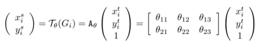
最右边式子左边的θ矩阵就是对应的采样矩阵。
STN 主要可以分为三个部分:
- Localisation net:是一个自己定义的网络,它输入U,输出变化参数ΘΘ,这个参数用来映射U和V的坐标关系
- Grid generator:根据V中的坐标点和变化参数ΘΘ,计算出U中的坐标点。这里是因为V的大小是自己先定义好的,当然可以得到V的所有坐标点,而填充V中每个坐标点的像素值的时候,要从U中去取,所以根据V中每个坐标点和变化参数ΘΘ进行运算,得到一个坐标。在sampler中就是根据这个坐标去U中找到像素值,这样子来填充V
- Sampler:要做的是填充V,根据Grid generator得到的一系列坐标和原图U(因为像素值要从U中取)来填充,因为计算出来的坐标可能为小数,要用另外的方法来填充,比如双线性插值。


class Net(nn.Module):
    def __init__(self):
        super(Net, self).__init__()
        self.conv1 = nn.Conv2d(1, 10, kernel_size=5)
        self.conv2 = nn.Conv2d(10, 20, kernel_size=5)
        self.conv2_drop = nn.Dropout2d()
        self.fc1 = nn.Linear(320, 50)
        self.fc2 = nn.Linear(50, 10)
        # Spatial transformer localization-network
        self.localization = nn.Sequential(
            nn.Conv2d(1, 8, kernel_size=7),
            nn.MaxPool2d(2, stride=2),
            nn.ReLU(True),
            nn.Conv2d(8, 10, kernel_size=5),
            nn.MaxPool2d(2, stride=2),
            nn.ReLU(True)
        )
       # Regressor for the 3 * 2 affine matrix
        self.fc_loc = nn.Sequential(
            nn.Linear(10 * 3 * 3, 32),
            nn.ReLU(True),
            nn.Linear(32, 3 * 2)
        )
       # Initialize the weights/bias with identity transformation
        self.fc_loc[2].weight.data.fill_(0)
        self.fc_loc[2].bias.data = torch.FloatTensor([1, 0, 0, 0, 1, 0])
    # Spatial transformer network forward function
    def stn(self, x):
        xs = self.localization(x)
        xs = xs.view(-1, 10 * 3 * 3)  #equal to reshape()  64x3x3x10-> 64*90
        theta = self.fc_loc(xs)   #64x6
        theta = theta.view(-1, 2, 3)  #reshape 64x2x3 Transform matrix
        grid = F.affine_grid(theta, x.size())
        #theta (Variable): input batch of affine matrices (N x 2 x 3)  64 x 2 x 3
        #size (torch.Size): the target output image size (N x C x H x W)  64x1x28x28
        #output (Variable): output Tensor of size (N x H x W x 2)         64x28x28x2
        x = F.grid_sample(x, grid)
        '''
        Args:
        input (Variable): input batch of images (N x C x IH x IW)
        grid (Variable): flow-field of size (N x OH x OW x 2)
        padding_mode (str): padding mode for outside grid values
            'zeros' | 'border'. Default: 'zeros'
        output: N x OH x OW x C
        '''
        return x  #64 x 28 x28 x 1

    def forward(self, x):  #x: 64 x28 x 28 x 1
        # transform the input
        x = self.stn(x)   # 64 x 28 x 28 x 1
        # Perform the usual forward pass
        x = F.relu(F.max_pool2d(self.conv1(x), 2))  # 64 x 12 x 12 x 10
        x = F.relu(F.max_pool2d(self.conv2_drop(self.conv2(x)), 2)) #64 x 4 x 4 x 20
        x = x.view(-1, 320)  #64x320
        x = F.relu(self.fc1(x)) #64x50
        x = F.dropout(x, training=self.training)
        x = self.fc2(x)  #64x10
        return F.log_softmax(x, dim=1)
1.2 通道域(Channel domain)
通道域的注意力机制原理很简单,我们可以从基本的信号变换的角度去理解。信号系统分析里面,任何一个信号其实都可以写成正弦波的线性组合,经过时频变换之后,时域上连续的正弦波信号就可以用一个频率信号数值代替了。

在卷积神经网络中,每一张图片初始会由(R,G,B)三通道表示出来,之后经过不同的卷积核之后,每一个通道又会生成新的信号,比如图片特征的每个通道使用64核卷积,就会产生64个新通道的矩阵(H,W,64),H,W分别表示图片特征的高度和宽度。
每个通道的特征其实就表示该图片在不同卷积核上的分量,类似于时频变换,而这里面用卷积核的卷积类似于信号做了傅里叶变换,从而能够将这个特征一个通道的信息给分解成64个卷积核上的信号分量。
既然每个信号都可以被分解成核函数上的分量,产生的新的64个通道对于关键信息的贡献肯定有多有少,如果我们给每个通道上的信号都增加一个权重,来代表该通道与关键信息的相关度的话,这个权重越大,则表示相关度越高,也就是我们越需要去注意的通道了。最后一届ImageNet冠军模型:SENet模型结构如下(《Squeeze-and-Excitation Networks》)

中间的模块就是SENet的创新部分,也就是注意力机制模块。这个注意力机制分成三个部分:挤压(squeeze),激励(excitation),以及注意(attention)。

很明显这个函数做了一个全局平均值,把每个通道内所有的特征值相加再平均,也是全局平均池化(global average pooling)的数学表达式。


这一步其实就是一个放缩的过程,不同通道的值乘上不同的权重,从而可以增强对关键通道域的注意力。

class SELayer(nn.Module):
    def __init__(self, channel, reduction=16):
        super(SELayer, self).__init__()
        self.avg_pool = nn.AdaptiveAvgPool2d(1)
        self.fc = nn.Sequential(
            nn.Linear(channel, channel // reduction, bias=False),
            nn.ReLU(inplace=True),
            nn.Linear(channel // reduction, channel, bias=False),
            nn.Sigmoid()
        )

    def forward(self, x):
        b, c, _, _ = x.size()  #batchsize,channel,height,width
        y = self.avg_pool(x).view(b, c)
        y = self.fc(y).view(b, c, 1, 1)
        return x * y.expand_as(x) #expand_as把一个tensor变成和函数括号内一样形状的tensor,用法与expand()类似
对于SE-ResNet模型,只需要将SE模块加入到残差单元就可以:
class SEBottleneck(nn.Module):
        expansion = 4

        def __init__(self, inplanes, planes, stride=1, downsample=None, reduction=16):
            super(SEBottleneck, self).__init__()
            self.conv1 = nn.Conv2d(inplanes, planes, kernel_size=1, bias=False)
            self.bn1 = nn.BatchNorm2d(planes)
            self.conv2 = nn.Conv2d(planes, planes, kernel_size=3, stride=stride,
                                   padding=1, bias=False)
            self.bn2 = nn.BatchNorm2d(planes)
            self.conv3 = nn.Conv2d(planes, planes * 4, kernel_size=1, bias=False)#1x1卷积核
            self.bn3 = nn.BatchNorm2d(planes * 4)
            self.relu = nn.ReLU(inplace=True)
            self.se = SELayer(planes * 4, reduction)
            self.downsample = downsample
            self.stride = stride

        def forward(self, x):
            residual = x

            out = self.conv1(x)
            out = self.bn1(out)
            out = self.relu(out)

            out = self.conv2(out)
            out = self.bn2(out)
            out = self.relu(out)

            out = self.conv3(out)
            out = self.bn3(out)
            out = self.se(out)

            if self.downsample is not None:
                residual = self.downsample(x)

            out += residual
            out = self.relu(out)

            return out
同理将SE模块加入Inception模块,其中Inception3函数可以直接import导包
class SEInception3(nn.Module):

    def __init__(self, num_classes, aux_logits=True, transform_input=False):

        super(SEInception3, self).__init__()
        model = Inception3(num_classes=num_classes, aux_logits=aux_logits,
                           transform_input=transform_input)
        model.Mixed_5b.add_module("SELayer", SELayer(192))
        model.Mixed_5c.add_module("SELayer", SELayer(256))
        model.Mixed_5d.add_module("SELayer", SELayer(288))
        model.Mixed_6a.add_module("SELayer", SELayer(288))
        model.Mixed_6b.add_module("SELayer", SELayer(768))
        model.Mixed_6c.add_module("SELayer", SELayer(768))
        model.Mixed_6d.add_module("SELayer", SELayer(768))
        model.Mixed_6e.add_module("SELayer", SELayer(768))
        if aux_logits:
            model.AuxLogits.add_module("SELayer", SELayer(768))
        model.Mixed_7a.add_module("SELayer", SELayer(768))
        model.Mixed_7b.add_module("SELayer", SELayer(1280))
        model.Mixed_7c.add_module("SELayer", SELayer(2048))
        self.model = model

    def forward(self, x):
        _, _, h, w = x.size()
        if (h, w) != (299, 299):
            raise ValueError("input size must be (299, 299)")
        return self.model(x)
顺便说一下SeNet的孪生SkNet(《Selective Kernel Networks》)
皮质神经元根据不同的刺激可动态调节其自身的感受野,因此,SkNet提出一种动态选择机制使每一个神经元可以针对目标物体的大小选择不同的感受野。SK单元包括三个方面:Split,Fuse,Select
Split:使用不同的卷积核对原图进行卷积;
Fuse:组合并聚积来自多个路径的信息,以获得选择权重的全局和综合表示;
Select:根据选择权重聚合不同大小的内核的特征映射。

class SKConv(nn.Module):
    def __init__(self,in_channels,out_channels,stride=1,M=2,r=16,L=32):
        '''
        :param in_channels:  输入通道维度
        :param out_channels: 输出通道维度   原论文中 输入输出通道维度相同
        :param stride:  步长,默认为1
        :param M:  分支数
        :param r: 特征Z的长度,计算其维度d 时所需的比率(论文中 特征S->Z 是降维,故需要规定 降维的下界)
        :param L:  论文中规定特征Z的下界,默认为32
        '''
        super(SKConv,self).__init__()
        d=max(in_channels//r,L)   # 计算向量Z 的长度d
        self.M=M
        self.out_channels=out_channels
        self.conv=nn.ModuleList()  # 根据分支数量 添加 不同核的卷积操作
        for i in range(M):
            # 为提高效率,原论文中 扩张卷积5x5为 (3X3,dilation=2)来代替。 且论文中建议组卷积G=32
            self.conv.append(nn.Sequential(nn.Conv2d(in_channels,out_channels,3,stride,padding=1+i,dilation=1+i,groups=32,bias=False),
                                           nn.BatchNorm2d(out_channels),
                                           nn.ReLU(inplace=True)))
        self.global_pool=nn.AdaptiveAvgPool2d(1) # 自适应pool到指定维度    这里指定为1,实现 GAP
        self.fc1=nn.Sequential(nn.Conv2d(out_channels,d,1,bias=False),
                               nn.BatchNorm2d(d),
                               nn.ReLU(inplace=True))   # 降维
        self.fc2=nn.Conv2d(d,out_channels*M,1,1,bias=False)  # 升维
        self.softmax=nn.Softmax(dim=1) # 指定dim=1  使得两个全连接层对应位置进行softmax,保证 对应位置a+b+..=1
    def forward(self, input):
        batch_size=input.size(0)
        output=[]
        #the part of split
        for i,conv in enumerate(self.conv):
            #print(i,conv(input).size())
            output.append(conv(input))
        #the part of fusion
        U=reduce(lambda x,y:x+y,output) # 逐元素相加生成 混合特征U
        s=self.global_pool(U)
        z=self.fc1(s)  # S->Z降维
        a_b=self.fc2(z) # Z->a,b 升维  论文使用conv 1x1表示全连接。结果中前一半通道值为a,后一半为b
        a_b=a_b.reshape(batch_size,self.M,self.out_channels,-1) #调整形状,变为 两个全连接层的值
        a_b=self.softmax(a_b) # 使得两个全连接层对应位置进行softmax
        #the part of selection
        a_b=list(a_b.chunk(self.M,dim=1))#split to a and b   chunk为pytorch方法,将tensor按照指定维度切分成 几个tensor块
        a_b=list(map(lambda x:x.reshape(batch_size,self.out_channels,1,1),a_b)) # 将所有分块  调整形状,即扩展两维
        V=list(map(lambda x,y:x*y,output,a_b)) # 权重与对应  不同卷积核输出的U 逐元素相乘
        V=reduce(lambda x,y:x+y,V) # 两个加权后的特征 逐元素相加
        return V
class SKBlock(nn.Module):
    '''
    基于Res Block构造的SK Block
    ResNeXt有  1x1Conv(通道数:x) +  SKConv(通道数:x)  + 1x1Conv(通道数:2x) 构成
    '''
    expansion=2 #指 每个block中 通道数增大指定倍数
    def __init__(self,inplanes,planes,stride=1,downsample=None):
        super(SKBlock,self).__init__()
        self.conv1=nn.Sequential(nn.Conv2d(inplanes,planes,1,1,0,bias=False),
                                 nn.BatchNorm2d(planes),
                                 nn.ReLU(inplace=True))
        self.conv2=SKConv(planes,planes,stride)
        self.conv3=nn.Sequential(nn.Conv2d(planes,planes*self.expansion,1,1,0,bias=False),
                                 nn.BatchNorm2d(planes*self.expansion))
        self.relu=nn.ReLU(inplace=True)
        self.downsample=downsample
    def forward(self, input):
        shortcut=input
        output=self.conv1(input)
        output=self.conv2(output)
        output=self.conv3(output)
        if self.downsample is not None:
            shortcut=self.downsample(input)
        output+=shortcut
        return self.relu(output)
class SKNet(nn.Module):
    '''
    参考 论文Table.1 进行构造
    '''
    def __init__(self,nums_class=1000,block=SKBlock,nums_block_list=[3, 4, 6, 3]):
        super(SKNet,self).__init__()
        self.inplanes=64
        # in_channel=3  out_channel=64  kernel=7x7 stride=2 padding=3
        self.conv=nn.Sequential(nn.Conv2d(3,64,7,2,3,bias=False),
                                nn.BatchNorm2d(64),
                                nn.ReLU(inplace=True))
        self.maxpool=nn.MaxPool2d(3,2,1) # kernel=3x3 stride=2 padding=1
        self.layer1=self._make_layer(block,128,nums_block_list[0],stride=1) # 构建表中 每个[] 的部分
        self.layer2=self._make_layer(block,256,nums_block_list[1],stride=2)
        self.layer3=self._make_layer(block,512,nums_block_list[2],stride=2)
        self.layer4=self._make_layer(block,1024,nums_block_list[3],stride=2)
        self.avgpool=nn.AdaptiveAvgPool2d(1) # GAP全局平均池化
        self.fc=nn.Linear(1024*block.expansion,nums_class) # 通道 2048 -> 1000
        self.softmax=nn.Softmax(-1) # 对最后一维进行softmax
    def forward(self, input):
        output=self.conv(input)
        output=self.maxpool(output)
        output=self.layer1(output)
        output=self.layer2(output)
        output=self.layer3(output)
        output=self.layer4(output)
        output=self.avgpool(output)
        output=output.squeeze(-1).squeeze(-1)
        output=self.fc(output)
        output=self.softmax(output)
        return output
    def _make_layer(self,block,planes,nums_block,stride=1):
        downsample=None
        if stride!=1 or self.inplanes!=planes*block.expansion:
            downsample=nn.Sequential(nn.Conv2d(self.inplanes,planes*block.expansion,1,stride,bias=False),
                                     nn.BatchNorm2d(planes*block.expansion))
        layers=[]
        layers.append(block(self.inplanes,planes,stride,downsample))
        self.inplanes=planes*block.expansion
        for _ in range(1,nums_block):
            layers.append(block(self.inplanes,planes))
        return nn.Sequential(*layers)
def SKNet50(nums_class=1000):
    return SKNet(nums_class,SKBlock,[3, 4, 6, 3]) # 论文通过[3, 4, 6, 3]搭配出SKNet50
def SKNet101(nums_class=1000):
    return SKNet(nums_class,SKBlock,[3, 4, 23, 3])
if __name__=='__main__':
    x = torch.rand(2, 3, 224, 224)
    model=SKNet50()
    y=model(x)
    print(y) # shape [2,1000]
每个SK单元由一个1x1的卷积,SK卷积,及1x1卷积组成,原网络中所有具有较大尺寸的卷积核都替换为SK卷积从而可以使网络选择合适的感受野大小。
