基本思想
所谓粒子滤波就是指:通过寻找一组在状态空间中传播的随机样本来近似的表示概率密度函数,用样本均值代替积分运算,进而获得系统状态的最小方差估计的过程,这些样本被形象的称为“粒子”,故而叫粒子滤波。采用数学语言描述如下: 对于平稳的随机过程, 假定k - 1 时刻系统的后验概率密度为p ( xk-1 zk-1 ) , 依据一定原则选取n 个随机样本点, k 时刻获得测量信息后, 经过状态和时间更新过程, n 个粒子的后验概率密度可近似为p ( xk zk ) 。随着粒子数目的增加, 粒子的概率密度函数逐渐逼近状态的概率密度函数, 粒子滤波估计即达到了最优贝叶斯估计的效果。
粒子滤波算法摆脱了解决非线性滤波问题时随机量必须满足高斯分布的制约条件, 并在一定程度上解决了粒子数样本匮乏问题, 因此近年来该算法在许多领域得到成功应用。
贝叶斯滤波
动态系统的状态空间模型可描述为
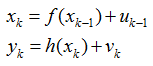
其中f(),h()分别为状态转移方程与观测方程,xk为系统状态,yk为观测值,uk为过程噪声,vk为观测噪声。为了描述方便,用Xk=x0:k={x0,x1,…,xk}与Yk=y0:k={y0,y1,…,yk}分别表示0到k时刻所有的状态与观测值。在处理目标跟踪问题时,通常假设目标的状态转移过程服从一阶马尔可夫模型,即当前时刻的状态xk只与上一时刻的状态xk-1有关。另外一个假设为观测值相互独立,即观测值yk只与k时刻的状态xk有关。
贝叶斯滤波为非线性系统的状态估计问题提供了一种基于概率分布形式的解决方案。贝叶斯滤波将状态估计视为一个概率推理过程,即将目标状态的估计问题转换为利用贝叶斯公式求解后验概率密度p(Xk|Yk)或滤波概率密度p(xk|Yk),进而获得目标状态的最优估计。贝叶斯滤波包含预测和更新两个阶段,预测过程利用系统模型预测状态的先验概率密度,更新过程则利用最新的测量值对先验概率密度进行修正,得到后验概率密度。
假设已知k-1时刻的概率密度函数为p(xk-1|Yk-1),贝叶斯滤波的具体过程如下:
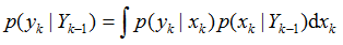
(1) 预测过程,由p(xk-1|Yk-1)得到p(xk|Yk-1):
p(xk,xk-1|Yk-1)=p(xk|xk-1,Yk-1)p(xk-1|Yk-1)
当给定xk-1时,状态xk与Yk-1相互独立,因此
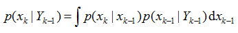
p(xk,xk-1|Yk-1)=p(xk|xk-1)p(xk-1|Yk-1)
上式两端对xk-1积分,可得Chapman-Komolgorov方程
(2) 更新过程,由p(xk|Yk-1)得到p(xk|Yk):
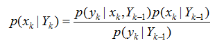
获取k时刻的测量yk后,利用贝叶斯公式对先验概率密度进行更新,得到后验概率
假设yk只由xk决定,即
p(yk|xk,Yk-1)=p(yk|xk)
因此
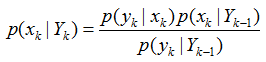
其中,p(yk|Yk-1)为归一化常数
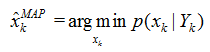
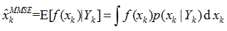
贝叶斯滤波以递推的形式给出后验(或滤波)概率密度函数的最优解。目标状态的最优估计值可由后验(或滤波)概率密度函数进行计算。通常根据极大后验(MAP)准则或最小均方误差(MMSE)准则,将具有极大后验概率密度的状态或条件均值作为系统状态的估计值,即
贝叶斯滤波需要进行积分运算,除了一些特殊的系统模型(如线性高斯系统,有限状态的离散系统)之外,对于一般的非线性、非高斯系统,贝叶斯滤波很难得到后验概率的封闭解析式。因此,现有的非线性滤波器多采用近似的计算方法解决积分问题,以此来获取估计的次优解。在系统的非线性模型可由在当前状态展开的线性模型有限近似的前提下,基于一阶或二阶Taylor级数展开的扩展Kalman滤波得到广泛应用。在一般情况下,逼近概率密度函数比逼近非线性函数容易实现。据此,Julier与Uhlmann提出一种Unscented Kalman滤波器,通过选定的sigma点来精确估计随机变量经非线性变换后的均值和方差,从而更好的近似状态的概率密度函数,其理论估计精度优于扩展Kalman滤波。获取次优解的另外一中方案便是基于蒙特卡洛模拟的粒子滤波器。
蒙特卡洛近似思想
蒙特卡洛积分是一项用随机釆样来估算积分值的技术,简单说就是以某事件出现的频率来指代该事件的概率。因此在滤波过程中,需要用到概率如P(x)的地方,一概对变量x采样,以大量采样及其相应的权值来近似表示P(x)。
然而,在计算机问世以前,随机试验却受到一定限制,这是因为要使计算结果的准确度足够高,需要进行的试验次数相当大。因此人们都认为随机试验要用人工进行冗长的计算,这实际上是不可能的。
随着电子计算机的出现,利用电子计算机可以实现大量的随机抽样试验,使得用随机试验方法解决实际问题才有了能。
它的基本思想是:为了求解数学、物理、工程技术以及生产管理等方面的问题,首先建立一个概率模型或随机过程,使它的参数等于问题的解,然后通过对模型或过程的观察或抽样试验来计算所求参数的统计特征,最后给出所求解的近似
值,而解的精确度可用估计值的标准误差来表示。
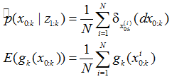
粒子滤波算法的核心思想便是利用一系列随机样本的加权和表示后验概率密度,通过求和来近似积分操作。
重要性采样 (Importance Sampling)
这是一种蒙特卡洛方法(Monte Carlo)。在有限的采样次数内,尽量让采样点覆盖对积分贡献很大的点。该方法目的并不是用来产生一个样本的,而是求一个函数的定积分的,只是因为该定积分的求法是通过对另一个叫容易采集分布的随机采用得到的。
序贯重要性采样(Sequential Importance Sainpling,SIS)
在粒子滤波算法中重采样的基本思想是抛弃那些对估计系统后验概率密度权值较小的粒子,通过复制权值较大的粒子来代替它们,进行重釆样有多种方法,常见的有多项式重釆样、系统重采样、分层抽样、残差抽样等,目前最为常用的重采样方法就是序贯重要性釆样。
在基于重要性重采样的蒙特卡洛模拟方法中,估计后验滤波概率需要利用所有的观测数据,每次新的观测数据来到都需要重新计算整个状态序列的重要性权值。序贯重要性釆样作为粒子滤波的基础,它将统计学的序贯分析方法应用到蒙特卡洛方法中,其主要思想就是递归的计算重采样粒子,通过保留以前所有采样时刻的粒子状态以保持采样粒子的继承性,从而实现后验滤波概率密度的递归估计。
基于序贯蒙特卡洛模拟方法的粒子滤波算法存在采样粒子权值退化问题以及计算量过大的问题,在实际计算中,经过数次迭代,只有少数粒子的权值较大,其余粒子的权值较小甚至可以忽略不计,粒子权值的方差随着时间的推移而增大,状态空间中的有效粒子数减少,随着无效粒子数量的增加,使得大量的计算消耗在对估计后验滤波概率分布几乎不起作用的粒子上,使得计算量增大且估计性能下降。
SIS算法的具体步骤如下:
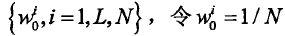
1.系统初始化
k = 0,随机提取N个样本点
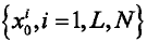
并给采样粒子赋予相应的初始权值为
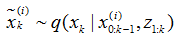
2.抽取N个样本
在时刻k=1,2,…,L通过随机釆样的方法从以下分布抽取N个样本
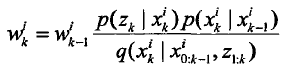
3.逐点计算对应的p(xk|xk-1)和p(zk|xk)
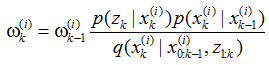
4.更新权值
该时刻的采样粒子点

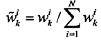
3.粒子权值归一化
权值退化
粒子滤波的核心思想是系统随机釆样与重要性重釆样的相加,粒子滤波首先根据系统在t时刻的系统状态x(t)和系统的概率分布生成大量的采样,这些采样就称之为粒子,那么这些采样在状态空间中的分布实际上就是x(t)的概率分布了,其后根据系统状态转移方程就可以对每一个粒子得到一个预测粒子,所有的预测粒子就代表系统所涉及的参数化东西。在滤波的预估计阶段,随机进行粒子采样,采样完成后根据特征相似度计算每个粒子的重要性,并根据重要性赋予粒子相应的权值,因此粒子滤波方法较之蒙特卡洛方法计算量较小,但是这种方法严重依赖于对初始状态的估计,随着迭代算法的进行,在经过数次迭代后其粒子采样的分配权重的方差会随着时间的推移而不断增大,除少数粒子以外的其他所有粒子只具有微小的权值并最终趋向于0,而少数粒子的权值会变的越来越大,随着采样过程的继续,最终所产生的粒子只是最初一小部分粒子权值的衍生,采样粒子代表的系统就会失去多样性,而当前系统的后验概率密度分布情况不能够有效的表示,我们将其称之为权值退化问题。
由于采样粒子权值退化问题在基于序贯重要性采样的粒子滤波算法中广泛存在,在经过数次迭代之后,许多粒子的权值变得很小,大量的计算浪费在小权值的粒子上,从而影响系统效率。目前降低该问题影响的最有效方法是选择重要性函数和采用重采样方法
重要性函数的选择
在重要性概率密度函数选择中融入系统最新的观测信息,通过选取好的重要性概率密度函数来有效抑制退化问题。
重采样
通过对粒子及其相应权值表示的概率密度函数进行重新采样,形成一个新的粒子集,该粒子集构成后验密度离散近似的一个经验分布,在釆样总数保持不变的情况下,权值较大的样本被多次复制,从而实现重釆样过程,通过引入重釆样技术,增加了权值较大的粒子数,在一定程度上能够有效解决粒子权值退化问题。重采样过程是以牺牲系统鲁棒性和计算效率来解决粒子权值退化问题的,并不是所有状态下的粒子都需要进行重采样,因此,我们需要进一步研究粒子权值的退化程度如何进行准确度量,并对粒子是否需要重采样进行有效判断。
重新采样获得的样本可以认为是一系列独立同分布的样本,其权重是一样的,均设为1/N。
采样贫乏
由于包含了大量重复的粒子(这些粒子具有高权值被多次选中),重采样导致了粒子多样性的丧失,此类问题在小噪声的环境下更加突出。事实上如果系统噪声非常小的话,所有粒子会在几次迭代之后崩塌为一个单独的粒子。
经典粒子滤波算法步骤
1.初始化:
取k=0,按p(x0)抽取N个样本点
2.重要性采样:
令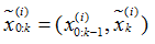
3.计算权值:
若采用一步转移后验状态分布,该式可简化为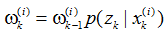
4.归一化权值:
t=

5.重采样:根据各自归一化权值

6.输出结果:算法的输出是粒子集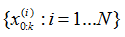

7.K=K+1,重复2步至6步。
粒子滤波其实质是利用一系列随机抽取的样本,也就是粒子,来替代状态的后验概率分布。当粒子的个数变得足够大时,通过这样的随机抽样方法就可以得到状态后验分布很好的近似。
<span style="font-size:18px;">function ParticleEx1

% Particle filter example, adapted from Gordon, Salmond, and Smith paper.

x = 0.1; % initial state
Q = 1; % process noise covariance
R = 1; % measurement noise covariance
tf = 50; % simulation length

N = 100; % number of particles in the particle filter

xhat = x;
P = 2;
xhatPart = x;

% Initialize the particle filter.
for i = 1 : N
    xpart(i) = x + sqrt(P) * randn;
end

xArr = [x];
yArr = [x^2 / 20 + sqrt(R) * randn];
xhatArr = [x];
PArr = [P];
xhatPartArr = [xhatPart];

close all;

for k = 1 : tf
    % System simulation
    x = 0.5 * x + 25 * x / (1 + x^2) + 8 * cos(1.2*(k-1)) + sqrt(Q) * randn;%状态方程
    y = x^2 / 20 + sqrt(R) * randn;%观测方程
    % Extended Kalman filter
    F = 0.5 + 25 * (1 - xhat^2) / (1 + xhat^2)^2;
    P = F * P * F' + Q;
    H = xhat / 10;
    K = P * H' * (H * P * H' + R)^(-1);
    xhat = 0.5 * xhat + 25 * xhat / (1 + xhat^2) + 8 * cos(1.2*(k-1));%预测
    xhat = xhat + K * (y - xhat^2 / 20);%更新
    P = (1 - K * H) * P;
    % Particle filter
    for i = 1 : N
        xpartminus(i) = 0.5 * xpart(i) + 25 * xpart(i) / (1 + xpart(i)^2) + 8 * cos(1.2*(k-1)) + sqrt(Q) * randn;
        ypart = xpartminus(i)^2 / 20;
        vhat = y - ypart;%观测和预测的差
        q(i) = (1 / sqrt(R) / sqrt(2*pi)) * exp(-vhat^2 / 2 / R);
    end
    % Normalize the likelihood of each a priori estimate.
    qsum = sum(q);
    for i = 1 : N
        q(i) = q(i) / qsum;%归一化权重
    end
    % Resample.
    for i = 1 : N
        u = rand; % uniform random number between 0 and 1
        qtempsum = 0;
        for j = 1 : N
            qtempsum = qtempsum + q(j);
            if qtempsum >= u
                xpart(i) = xpartminus(j);
                break;
            end
        end
    end
    % The particle filter estimate is the mean of the particles.
    xhatPart = mean(xpart);
    % Plot the estimated pdf's at a specific time.
    if k == 20
        % Particle filter pdf
        pdf = zeros(81,1);
        for m = -40 : 40
            for i = 1 : N
                if (m <= xpart(i)) && (xpart(i) < m+1)
                    pdf(m+41) = pdf(m+41) + 1;
                end
            end
        end
        figure;
        m = -40 : 40;
        plot(m, pdf / N, 'r');
        hold;
        title('Estimated pdf at k=20');
        disp(['min, max xpart(i) at k = 20: ', num2str(min(xpart)), ', ', num2str(max(xpart))]);
        % Kalman filter pdf
        pdf = (1 / sqrt(P) / sqrt(2*pi)) .* exp(-(m - xhat).^2 / 2 / P);
        plot(m, pdf, 'b');
        legend('Particle filter', 'Kalman filter');
    end
    % Save data in arrays for later plotting
    xArr = [xArr x];
    yArr = [yArr y];
    xhatArr = [xhatArr xhat];
    PArr = [PArr P];
    xhatPartArr = [xhatPartArr xhatPart];
end

t = 0 : tf;

%figure;
%plot(t, xArr);
%ylabel('true state');

figure;
plot(t, xArr, 'b.', t, xhatArr, 'k-', t, xhatArr-2*sqrt(PArr), 'r:', t, xhatArr+2*sqrt(PArr), 'r:');
axis([0 tf -40 40]);
set(gca,'FontSize',12); set(gcf,'Color','White');
xlabel('time step'); ylabel('state');
legend('True state', 'EKF estimate', '95% confidence region');

figure;
plot(t, xArr, 'b.', t, xhatPartArr, 'k-');
set(gca,'FontSize',12); set(gcf,'Color','White');
xlabel('time step'); ylabel('state');
legend('True state', 'Particle filter estimate');

xhatRMS = sqrt((norm(xArr - xhatArr))^2 / tf);
xhatPartRMS = sqrt((norm(xArr - xhatPartArr))^2 / tf);
disp(['Kalman filter RMS error = ', num2str(xhatRMS)]);
disp(['Particle filter RMS error = ', num2str(xhatPartRMS)]); </span>-
/** @file -
Definitions related to tracking with particle filtering -
@author Rob Hess -
@version 1.0.0-20060307 -
*/ -
#ifndef PARTICLES_H -
#define PARTICLES_H -
/******************************* Definitions *********************************/ -
/* standard deviations for gaussian sampling in transition model */ -
#define TRANS_X_STD 5.0 -
#define TRANS_Y_STD 5.0 -
#define TRANS_S_STD 0.001 -
/* autoregressive dynamics parameters for transition model */ -
#define A1 2.0 -
#define A2 -1.0 -
#define B0 1.0000 -
/* number of bins of HSV in histogram */ -
#define NH 10 -
#define NS 10 -
#define NV 10 -
/* max HSV values */ -
#define H_MAX 360.0 -
#define S_MAX 1.0 -
#define V_MAX 1.0 -
/* low thresholds on saturation and value for histogramming */ -
#define S_THRESH 0.1 -
#define V_THRESH 0.2 -
/* distribution parameter */ -
#define LAMBDA 20 -
#ifndef MIN -
# define MIN(a,b) ((a) > (b) ? (b) : (a)) -
#endif -
#ifndef MAX -
# define MAX(a,b) ((a) < (b) ? (b) : (a)) -
#endif -
//typedef unsigned char BYTE; -
class particle_filter -
{ -
private: -
typedef struct Rect -
{ -
int leftupx; -
int leftupy; -
int width; -
int height; -
Rect(){} -
Rect(int X, int Y, int W, int H) -
:leftupx(X), leftupy(Y), width(W), height(H) -
{} -
} -
Rect; -
struct Hsv -
{ -
double H;//0-360 -
double s;//0-1 -
double v;//0-1 -
}; -
/** -
An HSV histogram represented by NH * NS + NV bins. Pixels with saturation -
and value greater than S_THRESH and V_THRESH fill the first NH * NS bins. -
Other, "colorless" pixels fill the last NV value-only bins. -
*/ -
typedef struct histogram { -
float histo[NH*NS + NV]; /**< histogram array */ -
int n; /**< length of histogram array */ -
~histogram() -
{ -
//if (this) -
// delete this; -
} -
} histogram; -
/******************************* Structures **********************************/ -
/** -
A particle is an instantiation of the state variables of the system -
being monitored. A collection of particles is essentially a -
discretization of the posterior probability of the system. -
*/ -
typedef struct particle { -
float x; /**< current x coordinate */ -
float y; /**< current y coordinate */ -
float s; /**< scale */ -
float xp; /**< previous x coordinate */ -
float yp; /**< previous y coordinate */ -
float sp; /**< previous scale */ -
float x0; /**< original x coordinate */ -
float y0; /**< original y coordinate */ -
int width; /**< original width of region described by particle */ -
int height; /**< original height of region described by particle */ -
histogram* histo; /**< reference histogram describing region being tracked */ -
double w; /**< weight */ -
particle() -
{ -
s = 1; -
w = 0; -
} -
} particle; -
histogram** ref_histos;// -
unsigned int num_objects; -
Rect*target_rect_array;// -
unsigned int num_particles_for_each_object; -
particle** particles; -
Hsv*hsvimg; -
BYTE*RGBdata; -
unsigned int img_height; -
unsigned int img_width; -
bool isini; -
int current_frame; -
private: -
void draw_point(BYTE*rgbdata, int centerX, int centerY, COLORREF color,int linewidth); -
void copy_partile(const particle &src, particle&dst) -
{ -
dst.height = src.height; -
dst.histo = src.histo;//can be a problem memory leakage -
dst.s = src.s; -
dst.sp = src.sp; -
dst.w = src.w; -
dst.width = src.width; -
dst.x = src.x; -
dst.xp = src.xp; -
dst.x0 = src.x0; -
dst.y = src.y; -
dst.y0 = src.y0; -
dst.yp = src.yp; -
} -
/**************************** Function Prototypes ****************************/ -
/** -
Creates an initial distribution of particles by sampling from a Gaussian -
window around each of a set of specified locations -
@param regions an array of regions describing player locations around -
which particles are to be sampled -
@param histos array of histograms describing regions in \a regions -
@param n the number of regions in \a regions -
@param p the total number of particles to be assigned -
@return Returns an array of \a p particles sampled from around regions in -
\a regions -
*/ -
particle**& init_distribution(Rect* regions, histogram** histos); -
/** -
Samples a transition model for a given particle -
@param p a particle to be transitioned -
@param w video frame width -
@param h video frame height -
@param rng a random number generator from which to sample -
@return Returns a new particle sampled based on <EM>p</EM>'s transition -
model -
*/ -
particle transition(particle p, int w, int h); -
/** -
Normalizes particle weights so they sum to 1 -
@param particles an array of particles whose weights are to be normalized -
@param n the number of particles in \a particles -
*/ -
void normalize_weights(particle* particles, int n); -
/** -
Re-samples a set of weighted particles to produce a new set of unweighted -
particles -
@param particles an old set of weighted particles whose weights have been -
normalized with normalize_weights() -
@param n the number of particles in \a particles -
@return Returns a new set of unweighted particles sampled from \a particles -
*/ -
particle* resample(particle* particles, int n); -
/** -
Compare two particles based on weight. For use in qsort. -
@param p1 pointer to a particle -
@param p2 pointer to a particle -
@return Returns -1 if the \a p1 has lower weight than \a p2, 1 if \a p1 -
has higher weight than \a p2, and 0 if their weights are equal. -
*/ -
static int __cdecl particle_cmp(const void* p1,const void* p2); -
/** -
Displays a particle on an image as a rectangle around the region specified -
by the particle -
@param img the image on which to display the particle -
@param p the particle to be displayed -
@param color the color in which \a p is to be displayed -
*/ -
//void display_particle(IplImage* img, particle p, CvScalar color); -
/** -
Calculates the histogram bin into which an HSV entry falls -
@param h Hue -
@param s Saturation -
@param v Value -
@return Returns the bin index corresponding to the HSV color defined by -
\a h, \a s, and \a v. -
*/ -
int histo_bin(float h, float s, float v); -
/** -
Calculates a cumulative histogram as defined above for a given array -
of images -
@param imgs an array of images over which to compute a cumulative histogram; -
each must have been converted to HSV colorspace using bgr2hsv() -
@param n the number of images in imgs -
@return Returns an un-normalized HSV histogram for \a imgs -
*/ -
histogram* calc_histogram(Hsv*img, Rect rec); -
/** -
Normalizes a histogram so all bins sum to 1.0 -
@param histo a histogram -
*/ -
void normalize_histogram(histogram* histo); -
/** -
Computes squared distance metric based on the Battacharyya similarity -
coefficient between histograms. -
@param h1 first histogram; should be normalized -
@param h2 second histogram; should be normalized -
@return Rerns a squared distance based on the Battacharyya similarity -
coefficient between \a h1 and \a h2 -
*/ -
double histo_dist_sq(histogram* h1, histogram* h2); -
/** -
Computes the likelihood of there being a player at a given location in -
an image -
@param img image that has been converted to HSV colorspace using bgr2hsv() -
@param r row location of center of window around which to compute likelihood -
@param c col location of center of window around which to compute likelihood -
@param w width of region over which to compute likelihood -
@param h height of region over which to compute likelihood -
@param ref_histo reference histogram for a player; must have been -
normalized with normalize_histogram() -
@return Returns the likelihood of there being a player at location -
(\a r, \a c) in \a img -
*/ -
double likelihood(Hsv* img, int r, int c, -
int w, int h, histogram* ref_histo); -
/** -
Returns an image containing the likelihood of there being a player at -
each pixel location in an image -
@param img the image for which likelihood is to be computed; should have -
been converted to HSV colorspace using bgr2hsv() -
@param w width of region over which to compute likelihood -
@param h height of region over which to compute likelihood -
@param ref_histo reference histogram for a player; must have been -
normalized with normalize_histogram() -
@return Returns a single-channel, 32-bit floating point image containing -
the likelihood of every pixel location in \a img normalized so that the -
sum of likelihoods is 1. -
*/ -
double* likelihood_image(Hsv* img, int w, int h, histogram* ref_histo); -
/** -
Exports histogram data to a specified file. The file is formatted as -
follows (intended for use with gnuplot: -
Where n is the number of histogram bins and h_i, i = 1..n are -
floating point bin values -
@param histo histogram to be exported -
@param filename name of file to which histogram is to be exported -
@return Returns 1 on success or 0 on failure -
*/ -
int export_histogram(histogram* histo, char* filename); -
/* -
Computes a reference histogram for each of the object regions defined by -
the user -
@param frame video frame in which to compute histograms; should have been -
converted to hsv using bgr2hsv in observation.h -
@param regions regions of \a frame over which histograms should be computed -
@param n number of regions in \a regions -
@param export if TRUE, object region images are exported -
@return Returns an \a n element array of normalized histograms corresponding -
to regions of \a frame specified in \a regions. -
*/ -
histogram** compute_ref_histos(Hsv* frame, Rect* regions, int n); -
public: -
particle_filter(); -
~particle_filter(); -
void getHsvformRGBimg(BYTE*rgbdata, unsigned int W, unsigned int H); -
void get_target(RECT*target,int n); -
void track(); -
void init(); -
void track_single_frame(); -
}; -
#endif
-
#include "particle_filter.h" -
#include<cstdlib> -
#include<time.h> -
using namespace std; -
particle_filter::particle_filter() -
{ -
ref_histos = NULL; -
time_t t; -
srand(time(&t)); -
isini = true; -
current_frame = 0; -
} -
particle_filter::~particle_filter() -
{ -
for (int i = 0; i < num_objects; i++) -
{ -
free(particles[i]); -
free(ref_histos[i]); -
} -
free(particles); -
free(ref_histos); -
if (hsvimg) -
delete[]hsvimg; -
if (target_rect_array) -
delete[]target_rect_array; -
} -
double gaussrand() -
{ -
static double V1, V2, S; -
static int phase = 0; -
double X; -
if (phase == 0) { -
do { -
double U1 = (double)rand() / RAND_MAX; -
double U2 = (double)rand() / RAND_MAX; -
V1 = 2 * U1 - 1; -
V2 = 2 * U2 - 1; -
S = V1 * V1 + V2 * V2; -
} while (S >= 1 || S == 0); -
X = V1 * sqrt(-2 * log(S) / S); -
} -
else -
X = V2 * sqrt(-2 * log(S) / S); -
phase = 1 - phase; -
return X; -
} -
/*************************** Function Definitions ****************************/ -
/* -
Creates an initial distribution of particles at specified locations -
@param regions an array of regions describing player locations around -
which particles are to be sampled -
@param histos array of histograms describing regions in \a regions -
@param n the number of regions in \a regions -
@param p the total number of particles to be assigned -
@return Returns an array of \a p particles sampled from around regions in -
\a regions -
*/ -
particle_filter::particle**&particle_filter::init_distribution(Rect* regions, histogram** histos) -
{ -
//particle** particles; -
float x, y; -
int i, j, width, height; -
particles = (particle**)malloc(sizeof(particle*)*num_objects); -
for (int i = 0; i < num_objects; i++) -
particles[i] = (particle*)malloc(num_particles_for_each_object*sizeof(particle)); -
/* create particles at the centers of each of n regions */ -
for (i = 0; i < num_objects; i++) -
{ -
width = regions[i].width; -
height = regions[i].height; -
x = regions[i].leftupx + width / 2; -
y = regions[i].leftupy + height / 2; -
for (j = 0; j < num_particles_for_each_object; j++) -
{ -
int xx = target_rect_array[i].leftupx + target_rect_array[i].width / 2 + target_rect_array[i].width* gaussrand();;//x; -
if (xx < 0) -
xx = 0; -
if (xx >= img_width) -
xx = img_width - 1; -
particles[i][j].x0 = particles[i][j].xp = particles[i][j].x = xx; -
int yy = target_rect_array[i].leftupy + target_rect_array[i].height / 2 +target_rect_array[i].height* gaussrand();//y; -
if (yy < 0) -
yy = 0; -
if (yy >= img_height) -
yy = img_height - 1; -
particles[i][j].y0 = particles[i][j].yp = particles[i][j].y = yy; -
particles[i][j].sp = particles[i][j].s = 1.0; -
particles[i][j].width = width; -
particles[i][j].height = height; -
particles[i][j].histo = calc_histogram(hsvimg, Rect(particles[i][j].x - width / 2, -
particles[i][j].y - height / 2, width, height));//histos[i]; -
normalize_histogram(particles[i][j].histo); -
particles[i][j].w = 0; -
} -
} -
return particles; -
} -
/* -
Samples a transition model for a given particle -
@param p a particle to be transitioned -
@param w video frame width -
@param h video frame height -
@param rng a random number generator from which to sample -
@return Returns a new particle sampled based on <EM>p</EM>'s transition -
model -
*/ -
particle_filter::particle particle_filter::transition(particle p, int w, int h) -
{ -
float x, y, s; -
particle pn; -
#define PI 3.1415926 -
//double tt = 3; -
// sample new state using second-order autoregressive dynamics -
int sign = rand() % 2 == 0 ? 1 : -1; -
x = A1 * (p.x - p.x0) + A2 * (p.xp - p.x0) + -
sign*0.05*(double(rand()) / RAND_MAX)*p.width*p.s + p.x0;//B0 * 1.0 / sqrt(2 * PI) / TRANS_X_STD*exp(-pow(double(rand()) / RAND_MAX / TRANS_X_STD, 2)) + p.x0; -
pn.x = MAX(0.0, MIN((float)w - 1.0, x)); -
sign = rand() % 2 == 0 ? 1 : -1; -
y = A1 * (p.y - p.y0) + A2 * (p.yp - p.y0) + -
sign*0.05*(double(rand()) / RAND_MAX)*p.height*p.s + p.y0;//B0 * 1.0 / sqrt(2 * PI) / TRANS_Y_STD*exp(-pow(double(rand()) / RAND_MAX / TRANS_Y_STD, 2)) + p.y0; -
pn.y = MAX(0.0, MIN((float)h - 1.0, y)); -
//s = A1 * (p.s - 1.0) + A2 * (p.sp - 1.0) + -
// B0 * 1.0 / sqrt(2 * PI) / TRANS_S_STD*exp(-pow(double(rand()) / RAND_MAX / TRANS_S_STD, 2)) + 1.0; -
//pn.s = MAX(0.1, s); -
pn.s = 1; -
pn.xp = p.x; -
pn.yp = p.y; -
pn.sp = p.s; -
pn.x0 = p.x0; -
pn.y0 = p.y0; -
pn.width = p.width; -
pn.height = p.height; -
pn.histo = p.histo; -
pn.w = 0; -
//assert(p.width == target_rect_array[0].width); -
return pn; -
} -
/* -
Normalizes particle weights so they sum to 1 -
@param particles an array of particles whose weights are to be normalized -
@param n the number of particles in \a particles -
*/ -
void particle_filter::normalize_weights(particle* particles, int n) -
{ -
double sum = 0; -
int i; -
double maxweight = 0; -
for (i = 0; i < n; i++) -
sum += particles[i].w; -
for (i = 0; i < n; i++) -
{ -
particles[i].w /= sum; -
if (particles[i].w>maxweight) -
maxweight = particles[i].w; -
} -
} -
/* -
Compare two particles based on weight. For use in qsort. -
@param p1 pointer to a particle -
@param p2 pointer to a particle -
@return Returns -1 if the \a p1 has lower weight than \a p2, 1 if \a p1 -
has higher weight than \a p2, and 0 if their weights are equal. -
*/ -
int __cdecl particle_filter::particle_cmp(const void* p1, const void* p2) -
{ -
particle* _p1 = (particle*)p1; -
particle* _p2 = (particle*)p2; -
if (_p1->w > _p2->w) -
return -1; -
if (_p1->w < _p2->w) -
return 1; -
return 0; -
} -
/* -
Re-samples a set of particles according to their weights to produce a -
new set of unweighted particles -
@param particles an old set of weighted particles whose weights have been -
normalized with normalize_weights() -
@param n the number of particles in \a particles -
@return Returns a new set of unweighted particles sampled from \a particles -
*/ -
particle_filter::particle*particle_filter::resample(particle* particles, int n) -
{ -
particle* new_particles; -
int i, j, np, k = 0; -
qsort(particles, n, sizeof(particle), &particle_cmp); -
int nnn = 0.03*num_particles_for_each_object; -
int kk = 0; -
new_particles = (particle*)malloc(sizeof(particle)*n); -
int count = 0; -
int max_dis = (particles[0].height + particles[0].width); -
int cnt = 0; -
int maxnum = 0; -
for (i = 0; i < n; i++) -
{ -
np = round(particles[i].w * n); -
//if (np <= 0) -
// np = 1; -
if (i == 0 && np < 30) -
np = 30; -
for (j = 0; j < np; j++) -
{ -
//new_particles[k++] = particles[i]; -
double dis = abs(particles[i].x - particles[0].x) + abs(particles[i].y - particles[0].y); -
if ( dis> max_dis/3) -
{ -
copy_partile(particles[kk++%nnn], new_particles[k]); -
cnt++; -
} -
else -
copy_partile(particles[i], new_particles[k]); -
k++; -
if (k == n) -
goto exit; -
count++; -
} -
} -
for (int i = k; i < n; i++) -
copy_partile(particles[kk++%nnn], new_particles[i]); -
///while (k < n) -
// new_particles[k++] = particles[0]; -
exit: -
return new_particles; -
} -
/* -
Displays a particle on an image as a rectangle around the region specified -
by the particle -
@param img the image on which to display the particle -
@param p the particle to be displayed -
@param color the color in which \a p is to be displayed -
*/ -
/*void particle_filter::display_particle(IplImage* img, particle p, CvScalar color) -
{ -
int x0, y0, x1, y1; -
x0 = round(p.x - 0.5 * p.s * p.width); -
y0 = round(p.y - 0.5 * p.s * p.height); -
x1 = x0 + round(p.s * p.width); -
y1 = y0 + round(p.s * p.height); -
//Rectangle(img, cvPoint(x0, y0), cvPoint(x1, y1), color, 1, 8, 0); -
}*/ -
/* -
Calculates the histogram bin into which an HSV entry falls -
@param h Hue -
@param s Saturation -
@param v Value -
@return Returns the bin index corresponding to the HSV color defined by -
\a h, \a s, and \a v. -
*/ -
int particle_filter::histo_bin(float h, float s, float v) -
{ -
int hd, sd, vd; -
/* if S or V is less than its threshold, return a "colorless" bin */ -
vd = MIN((int)(v * NV / V_MAX), NV - 1); -
if (s < S_THRESH || v < V_THRESH) -
return NH * NS + vd; -
/* otherwise determine "colorful" bin */ -
hd = MIN((int)(h * NH / H_MAX), NH - 1); -
sd = MIN((int)(s * NS / S_MAX), NS - 1); -
return sd * NH + hd; -
} -
/* -
Calculates a cumulative histogram as defined above for a given array -
of images -
@param img an array of images over which to compute a cumulative histogram; -
each must have been converted to HSV colorspace using bgr2hsv() -
@param n the number of images in imgs -
@return Returns an un-normalized HSV histogram for \a imgs -
*/ -
particle_filter::histogram* particle_filter::calc_histogram(Hsv*img, Rect rec) -
{ -
//IplImage* img; -
histogram* histo; -
//correct window -
int leftup_X = rec.leftupx; -
int leftup_Y =rec.leftupy; -
if (leftup_X < 0) -
leftup_X = 0; -
if (leftup_X >= img_width - rec.width) -
leftup_X = img_width - rec.width - 1; -
if (leftup_Y < 0) -
leftup_Y = 0; -
if (leftup_Y >= img_height - rec.height) -
leftup_Y = img_height - rec.height - 1; -
Rect rect(leftup_X, leftup_Y, rec.width, rec.height); -
float* hist; -
int i, r, c, bin; -
int size = sizeof(histogram); -
histo = (histogram*)malloc(sizeof(histogram)); -
histo->n = NH*NS + NV; -
hist = histo->histo; -
memset(hist, 0, histo->n * sizeof(float)); -
/* extract individual HSV planes from image */ -
/* increment appropriate histogram bin for each pixel */ -
for (r = 0; r < rect.height; r++) -
for (c = 0; c < rect.width; c++) -
{ -
bin = histo_bin( /*pixval32f( h, r, c )*/img[img_width*(rect.leftupy + r) + rect.leftupx + c].H, -
img[img_width*(rect.leftupy + r) + rect.leftupx + c].s, -
img[img_width*(rect.leftupy + r) + rect.leftupx + c].v); -
hist[bin] += 1; -
} -
return histo; -
} -
/* -
Normalizes a histogram so all bins sum to 1.0 -
@param histo a histogram -
*/ -
void particle_filter::normalize_histogram(histogram* histo) -
{ -
float* hist; -
float sum = 0, inv_sum; -
int i, n; -
hist = histo->histo; -
n = histo->n; -
/* compute sum of all bins and multiply each bin by the sum's inverse */ -
for (i = 0; i < n; i++) -
sum += hist[i]; -
inv_sum = 1.0 / sum; -
for (i = 0; i < n; i++) -
hist[i] *= inv_sum; -
} -
/* -
Computes squared distance metric based on the Battacharyya similarity -
coefficient between histograms. -
@param h1 first histogram; should be normalized -
@param h2 second histogram; should be normalized -
@return Returns a squared distance based on the Battacharyya similarity -
coefficient between \a h1 and \a h2 -
*/ -
double particle_filter::histo_dist_sq(histogram* h1, histogram* h2) -
{ -
float* hist1, *hist2; -
double sum = 0; -
int i, n; -
n = h1->n; -
hist1 = h1->histo; -
hist2 = h2->histo; -
/* -
According the the Battacharyya similarity coefficient, -
D = \sqrt{ 1 - \sum_1^n{ \sqrt{ h_1(i) * h_2(i) } } } -
*/ -
for (i = 0; i < n; i++) -
sum += sqrt(hist1[i] * hist2[i]); -
return 1.0 - sum; -
} -
/* -
Computes the likelihood of there being a player at a given location in -
an image -
@param img image that has been converted to HSV colorspace using bgr2hsv() -
@param r row location of center of window around which to compute likelihood -
@param c col location of center of window around which to compute likelihood -
@param w width of region over which to compute likelihood -
@param h height of region over which to compute likelihood -
@param ref_histo reference histogram for a player; must have been -
normalized with normalize_histogram() -
@return Returns the likelihood of there being a player at location -
(\a r, \a c) in \a img -
*/ -
double particle_filter::likelihood(Hsv* img, int r, int c, -
int w, int h, histogram* ref_histo) -
{ -
//IplImage* tmp; -
histogram* histo; -
float d_sq; -
//correct window -
int leftup_X = c - w / 2; -
int leftup_Y = r - h / 2; -
if (leftup_X < 0) -
leftup_X = 0; -
if (leftup_X >= img_width - w) -
leftup_X = img_width - w - 1; -
if (leftup_Y < 0) -
leftup_Y = 0; -
if (leftup_Y >= img_height - h) -
leftup_Y = img_height - h - 1; -
Rect rec(leftup_X, leftup_Y, w, h); -
histo = calc_histogram(img, rec); -
normalize_histogram(histo); -
/* compute likelihood as e^{\lambda D^2(h, h^*)} */ -
d_sq = histo_dist_sq(histo, ref_histo); -
free(histo); -
double re = exp(-LAMBDA * d_sq); -
return re; -
} -
/* -
Returns an image containing the likelihood of there being a player at -
each pixel location in an image -
@param img the image for which likelihood is to be computed; should have -
been converted to HSV colorspace using bgr2hsv() -
@param w width of region over which to compute likelihood -
@param h height of region over which to compute likelihood -
@param ref_histo reference histogram for a player; must have been -
normalized with normalize_histogram() -
@return Returns a single-channel, 32-bit floating point image containing -
the likelihood of every pixel location in \a img normalized so that the -
sum of likelihoods is 1. -
*/ -
double* particle_filter::likelihood_image(Hsv* img, int w, int h, histogram* ref_histo) -
{ -
double* l, *l2; -
double sum = 0; -
int i, j; -
l = new double[img_height*img_width]; -
for (i = 0; i < img_height; i++) -
for (j = 0; j < img_width; j++) -
{ //setpix32f( l, i, j, likelihood( img, i, j, w, h, ref_histo ) ); -
l[i*img_width + j] = likelihood(img, i, j, w, h, ref_histo); -
sum += l[i*img_width + j]; -
} -
for (i = 0; i < img_height; i++) -
for (j = 0; j < img_width; j++) -
{ -
l[i*img_width + j] /= sum; -
} -
return l; -
} -
/* -
Exports histogram data to a specified file. The file is formatted as -
follows (intended for use with gnuplot: -
Where n is the number of histogram bins and h_i, i = 1..n are -
floating point bin values -
@param histo histogram to be exported -
@param filename name of file to which histogram is to be exported -
@return Returns 1 on success or 0 on failure -
*/ -
int particle_filter::export_histogram(histogram* histo, char* filename) -
{ -
int i, n; -
float* h; -
FILE* file = fopen(filename, "w"); -
if (!file) -
return 0; -
n = histo->n; -
h = histo->histo; -
for (i = 0; i < n; i++) -
fprintf(file, "%d %f\n", i, h[i]); -
fclose(file); -
return 1; -
} -
//RGBdata不需要排列成BGRBGR的格式,原始数据就行 -
void particle_filter::getHsvformRGBimg(BYTE*RGBdata, unsigned int W, unsigned int H) -
{ -
this->RGBdata = RGBdata; -
#define LINEWIDTH(bits) (((bits) + 31) / 32 * 4) -
int nSrcLine = LINEWIDTH(W * 24); -
if (isini) -
{ -
isini = false; -
img_height = H; -
img_width = W; -
hsvimg = new Hsv[W*H]; -
} -
else -
if (W != img_height || H != img_height) -
{ -
delete[]hsvimg; -
hsvimg = new Hsv[W*H]; -
img_height = H; -
img_width = W; -
} -
for (int i = 0; i < img_height; i++) -
for (int j = 0; j < img_width; j++) -
{ -
float min, max,r,g,b; -
r = RGBdata[i*nSrcLine + j * 3 + 2]; -
g = RGBdata[i*nSrcLine + j * 3 + 1]; -
b = RGBdata[i*nSrcLine + j * 3 ]; -
float delta; -
float tmp = min(r, g); -
min = min(tmp, b); -
tmp = max(r, g); -
max = max(tmp, b); -
//min = MIN(r, g, b); -
//max = MAX(r, g, b); -
hsvimg[img_width*i + j].v = max; // v -
delta = max - min; -
if (max != 0) -
{ -
hsvimg[img_width*i+j].s = delta / max; // s -
} -
else -
{ -
// r = g = b = 0 // s = 0, v is undefined -
hsvimg[img_width*i + j].s = 0; -
//hsvimg[img_width*i + j].H = -1; -
} -
if (max == min) -
{ -
hsvimg[img_width*i + j].H = 0; -
} -
else if (r == max) -
{ -
hsvimg[img_width*i + j].H = (g - b) / delta; // between yellow & magenta -
} -
else if (g == max) -
{ -
hsvimg[img_width*i + j].H = 2 + (b - r) / delta; // between cyan & yellow -
} -
else -
{ -
hsvimg[img_width*i + j].H = 4 + (r - g) / delta; // between magenta & cyan -
} -
hsvimg[img_width*i + j].H *= 60; // degrees -
if (hsvimg[img_width*i + j].H < 0) -
{ -
hsvimg[img_width*i + j].H += 360; -
} -
if (hsvimg[img_width*i + j].H > 360) -
{ -
hsvimg[img_width*i + j].H = hsvimg[img_width*i + j].H - 360; -
} -
} -
} -
particle_filter::histogram** particle_filter::compute_ref_histos(Hsv* frame, Rect* regions, int n) -
{ -
histogram** histos = (histogram**)malloc(n * sizeof(histogram*)); -
int i; -
/* extract each region from frame and compute its histogram */ -
for (i = 0; i < n; i++) -
{ -
histos[i] = calc_histogram(frame, regions[i]); -
normalize_histogram(histos[i]); -
} -
return histos; -
} -
void particle_filter::init() -
{ -
num_particles_for_each_object = 500; -
ref_histos = compute_ref_histos(hsvimg, target_rect_array, num_objects); -
init_distribution(target_rect_array, ref_histos); -
} -
void particle_filter::track_single_frame() -
{ -
current_frame++; -
for (int i = 0; i < num_objects; i++) -
{/* perform prediction and measurement for each particle */ -
for (int j = 0; j < num_particles_for_each_object; j++) -
{ -
particles[i][j] = transition(particles[i][j], img_width, img_height); -
double s = particles[i][j].s; -
//assert(int(particles[i][j].width * s) == target_rect_array[i].width); -
//assert(int(particles[i][j].height * s) == target_rect_array[i].height); -
//if (particles[i][j].width != target_rect_array[i].width) -
// particles[i][j].width = target_rect_array[i].width; -
//if (particles[i][j].height != target_rect_array[i].height) -
// particles[i][j].height = target_rect_array[i].height; -
particles[i][j].w = likelihood(hsvimg, -
round(particles[i][j].y),//center of window -
round(particles[i][j].x),//center of window -
round(particles[i][j].width * s), -
round(particles[i][j].height * s), -
ref_histos[i]); -
} -
/* normalize weights and resample a set of unweighted particles */ -
normalize_weights(particles[i], num_particles_for_each_object); -
particle* new_particles = resample(particles[i], num_particles_for_each_object); -
free(particles[i]); -
particles[i] = new_particles; -
/* display all particles if requested */ -
qsort(particles[i], num_particles_for_each_object, sizeof(particle), &particle_cmp); -
//display result -
COLORREF color = RGB(255, 255, 255); -
for (int j = 0; j < num_particles_for_each_object; j++) -
{ -
draw_point(this->RGBdata, particles[i][j].x, particles[i][j].y, color, 5); -
} -
color = RGB(0, 255, 0); -
draw_point(this->RGBdata, particles[i][0].x, particles[i][0].y, color, 15); -
if (current_frame % 2 == 0) -
// init_distribution(target_rect_array, ref_histos); -
//update model -
{ -
double s = particles[i][0].s; -
int leftup_X = particles[i][0].x - particles[i][0].width*s / 2; -
int leftup_Y = particles[i][0].y - particles[i][0].height*s / 2; -
if (leftup_X < 0) -
leftup_X = 0; -
if (leftup_X >= img_width - particles[i][0].width*s) -
leftup_X = img_width - particles[i][0].width*s - 1; -
if (leftup_Y < 0) -
leftup_Y = 0; -
if (leftup_Y >= img_height - particles[i][0].height*s) -
leftup_Y = img_height - particles[i][0].height*s - 1; -
Rect rec(leftup_X, leftup_Y, particles[i][0].width*s, particles[i][0].height*s); -
histogram*newhist = calc_histogram(hsvimg, rec); -
normalize_histogram(newhist); -
//delete[]ref_histos[i]; -
for (int j = 0; j < ref_histos[i]->n; j++) -
ref_histos[i]->histo[j] = newhist->histo[j]; -
delete newhist; -
} -
} -
} -
void particle_filter::draw_point(BYTE*rgbdata, int centerX, int centerY, COLORREF clo, int linewidth) -
{ -
assert(rgbdata); -
//#define LINEWIDTH(bits) (((bits) + 31) / 32 * 4) -
int nSrcLine = LINEWIDTH(img_width * 24); -
for (int j = -linewidth; j < linewidth + 1; j++) -
{ -
if (centerX + j >= 0 && centerX + j < img_width) -
{ -
rgbdata[centerY*nSrcLine + 3 * (centerX + j)] = GetBValue(clo); -
rgbdata[centerY*nSrcLine + 3 * (centerX + j) + 1] = GetGValue(clo); -
rgbdata[centerY*nSrcLine + 3 * (centerX + j) + 2] = GetRValue(clo); -
rgbdata[(centerY-1)*nSrcLine + 3 * (centerX + j)] = GetBValue(clo); -
rgbdata[(centerY-1)*nSrcLine + 3 * (centerX + j) + 1] = GetGValue(clo); -
rgbdata[(centerY-1)*nSrcLine + 3 * (centerX + j) + 2] = GetRValue(clo); -
} -
} -
for (int j = -linewidth; j < linewidth + 1; j++) -
{ -
if (centerY + j >= 0 && centerY + j < img_height) -
{ -
rgbdata[(centerY + j)*nSrcLine + 3 * centerX] = GetBValue(clo); -
rgbdata[(centerY + j)*nSrcLine + 3 * centerX + 1] = GetGValue(clo); -
rgbdata[(centerY + j)*nSrcLine + 3 * centerX + 2] = GetRValue(clo); -
rgbdata[(centerY + j)*nSrcLine + 3 * centerX-3] = GetBValue(clo); -
rgbdata[(centerY + j)*nSrcLine + 3 * centerX -2] = GetGValue(clo); -
rgbdata[(centerY + j)*nSrcLine + 3 * centerX -1] = GetRValue(clo); -
} -
} -
} -
void particle_filter::get_target(RECT*target,int n) -
{ -
assert(target); -
num_objects = n; -
target_rect_array = new Rect[n]; -
for (int i = 0; i < n; i++) -
{ -
target_rect_array[i].leftupy = target[i].top; -
target_rect_array[i].leftupx = target[i].left; -
target_rect_array[i].width = target[i].right-target[i].left; -
target_rect_array[i].height = target[i].bottom - target[i].top; -
} -
}
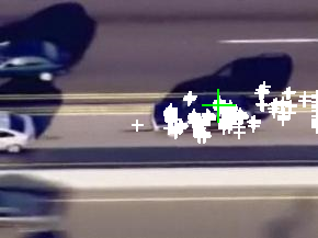
下面是我实现的跟踪结果,白色十字代表粒子,绿色大十字代表目标最可能的位置。
如何理解 重要性采样(importance sampling)
