凸集和凸函数

CMU凸优化笔记–凸集和凸函数

结束了一段时间的学习任务，于是打算做个总结。主要内容都是基于CMU的Ryan Tibshirani开设的Convex Optimization课程做的笔记。这里只摘了部分内容做了笔记，很感谢Ryan Tibshirani在官网中所作的课程内容开源。也很感谢韩龙飞在CMU凸优化课程中的中文笔记，我在其基础上做了大量的内容参考。才疏学浅，忘不吝赐教。

1、凸集合

1.1 基本概念

定义：给定一个集合C⊆Rn” role=”presentation” style=”position: relative;”>C⊆Rn,满足下列条件则称为凸集

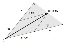
x,y∈C⇒tx+(1−t)y∈C” role=”presentation” style=”position: relative;”>x,y∈C⇒tx+(1−t)y∈C

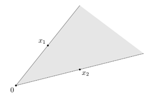
直观上看，可以利用下图帮助理解，假定我们的变量在二维空间中，x,y” role=”presentation” style=”position: relative;”>x,y张成的集合空间中。

那么从定义出发，我们也能知道非凸集的情况，下图左侧为凸集，右图为非凸集

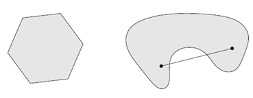
一句话来概括凸集就是集合内任意两点间连线依旧在集合内。

扫描二维码关注公众号，回复： 10786517 查看本文章

1.2 凸集简单例子

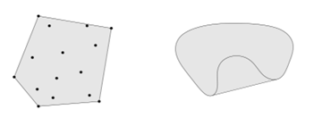
凸包(convex hull)：给定集合内的任意k” role=”presentation” style=”position: relative;”>k,任意的线性组合形式：

θ1x1+...+θkxk,θi≤,i=1,...,k” role=”presentation” style=”position: relative;”>θ1x1+...+θkxk,θi≤,i=1,...,k。convex hull总是凸的。可以直观认为凸包就是最外围的元素所围成的集合外壳，下图是两个凸包的例子：

空集、点、线都是凸集合
范数球（Norm ball）: 半径为r” role=”presentation” style=”position: relative;”>r
超平面（Hyperplane）: 给定任意a,b” role=”presentation” style=”position: relative;”>a,b
半空间（Half space）: {x:aTx≤b}” role=”presentation” style=”position: relative;”>{x:aTx≤b}
仿射空间(Affine space):{x:Ax=b}” role=”presentation” style=”position: relative;”>{x:Ax=b}
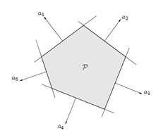
多面体(Polyhedron):{x:Ax≤b}” role=”presentation” style=”position: relative;”>{x:Ax≤b}，下图为多面体

Note:集合{x:Ax≤b,Cx=d}” role=”presentation” style=”position: relative;”>{x:Ax≤b,Cx=d}也是一个Polyhedron吗？

Answer:是的。因为对于任意的Cx=d” role=”presentation” style=”position: relative;”>Cx=d形式一致。

1.3 锥（Cone）：

定义：给定C∈Rn” role=”presentation” style=”position: relative;”>C∈Rn称之为锥。

凸锥（convex cone）：x1,x2∈C⇒t1x1+t2x2∈C” role=”presentation” style=”position: relative;”>x1,x2∈C⇒t1x1+t2x2∈C为凸锥。显然凸锥是锥的一种。

例子：

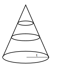
范数锥(Norm cone):{(x,t):||x||≤t}” role=”presentation” style=”position: relative;”>{(x,t):||x||≤t}做出了三维情况下的图：

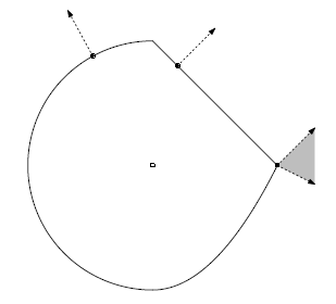
正规锥(Normal cone):给定任意集合C” role=”presentation” style=”position: relative;”>C,定义：

Nc(x)={g:gTx≥gTy,foranyy∈C}” role=”presentation” style=”position: relative;”>Nc(x)={g:gTx≥gTy,foranyy∈C}

其含义是指Normal cone中的点与集合C” role=”presentation” style=”position: relative;”>C内的点的内积永远大于集合内任意点与Normal cone内点的内积。如下图所示：

1.4 凸集的一些特性

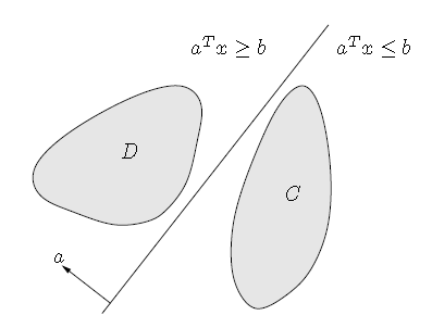
可分离超平面理论（Separating hyperplane theorem）：两个不相交的凸集总存在一个超平面能将两者分离，如果C⋂D=∅” role=”presentation” style=”position: relative;”>C⋂D=∅使得有:

C⊆{x:aTx≤b}” role=”presentation” style=”position: relative;”>C⊆{x:aTx≤b}。如下图所示：

支撑超平面理论(Supporting hyperplane theorem):凸集边界上的一点必然存在一个支撑超平面穿过该点，即如果C” role=”presentation” style=”position: relative;”>C。如下图：

1.5 保凸操作

集合交（Intersection）：任何凸集之交产生的集合依旧是凸集。
缩放和平移（Scaling and translation）：假设C” role=”presentation” style=”position: relative;”>C也是凸的。
仿射映射与预映射(Affine images and preimages)：如果f(x)=Ax+b” role=”presentation” style=”position: relative;”>f(x)=Ax+b也是凸的。

1.6 凸集与保凸操作相关例子

条件概率集合(conditional probability set)：U,V” role=”presentation” style=”position: relative;”>U,V

2 、凸函数

2.1 基本概念

定义：给定映射f:Rn→R” role=”presentation” style=”position: relative;”>f:Rn→R为凸集，那么

f(tx+(1−t)y)≤tf(x)+(1−t)f(y)” role=”presentation” style=”position: relative;”>f(tx+(1−t)y)≤tf(x)+(1−t)f(y)。如下图：

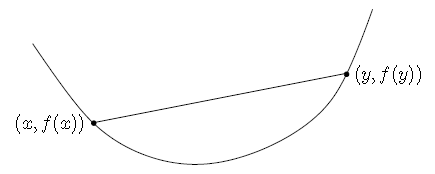
从上图可以看出，f” role=”presentation” style=”position: relative;”>f之间的直线下方。

Note:

严格凸(Strictly convex):对于任意x≠y” role=”presentation” style=”position: relative;”>x≠y比线性函数要更弯曲
强凸(Strongly convex):对于参数m>0” role=”presentation” style=”position: relative;”>m>0要比一般的二次函数要弯曲。
强凸 ⇒” role=”presentation” style=”position: relative;”>⇒ 凸

2.2 凸函数例子

单变量函数：

例如指数函数eax” role=”presentation” style=”position: relative;”>eax是非凸函数

仿射函数(Affine function):

aTx+b” role=”presentation” style=”position: relative;”>aTx+b既是凸函数又是非凸函数

二次函数(Quadratic function)：

12xTQx+bTx+c” role=”presentation” style=”position: relative;”>12xTQx+bTx+c（半正定）的时候为凸

最小平方损失函数（Least squares loss）:

||y−Ax||22” role=”presentation” style=”position: relative;”>||y−Ax||22总是半正定的

范数(Norm)：

||x||” role=”presentation” style=”position: relative;”>||x||。

谱(spectral)范数：∥X∥op=σ1(X)” role=”presentation” style=”position: relative;”>∥X∥op=σ1(X),

核范数（nuclear）:||X||tr=∑i=1rσr(X)” role=”presentation” style=”position: relative;”>||X||tr=∑ri=1σr(X)的从大到小排序的奇异值。

指示函数(Indicator function):

如果C” role=”presentation” style=”position: relative;”>C为凸函数。

最大值函数（Max function）:

f(x)=max{x1,...,xn}” role=”presentation” style=”position: relative;”>f(x)=max{x1,...,xn}为凸函数

2.3 凸函数的一些特性

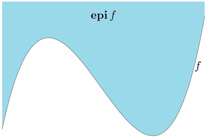
上镜特性(Epigraph characterization):函数f” role=”presentation” style=”position: relative;”>f为凸集，如下图：

一阶特性(First-order characterization):假设f” role=”presentation” style=”position: relative;”>f。

Note:如何证明凸函数的一阶特性？

Answer:从凸函数定义出发，f(ty+(1−t)x)≤tf(y)+(1−t)f(x)⇒f(t(y−x)+x)+f(x))≤t(f(y)−f(x))+f(x)⇒f(t(y−x)+x)−f(x)t(y−x)≤fracf(y)−f(x)y−x⇒limt→0f(t(y−x)+x)−f(x)t(y−x)=∇f(x)⇒∇f(x)(y−x)≤f(y)−f(x)⇒f(y)≥f(x)+∇f(x)(y−x)” role=”presentation” style=”position: relative;”>f(ty+(1−t)x)≤tf(y)+(1−t)f(x)⇒f(t(y−x)+x)+f(x))≤t(f(y)−f(x))+f(x)⇒f(t(y−x)+x)−f(x)t(y−x)≤fracf(y)−f(x)y−x⇒limt→0f(t(y−x)+x)−f(x)t(y−x)=∇f(x)⇒∇f(x)(y−x)≤f(y)−f(x)⇒f(y)≥f(x)+∇f(x)(y−x)

二阶特性：如果函数二阶可微分，则f” role=”presentation” style=”position: relative;”>f
Jensen不等式：假若f” role=”presentation” style=”position: relative;”>f

2.4保凸操作

非负线性组合

f1,...,fm” role=”presentation” style=”position: relative;”>f1,...,fm为凸。

逐点最大化

如果fs” role=”presentation” style=”position: relative;”>fs是凸函数。

部分最小化

如果g(x,y)” role=”presentation” style=”position: relative;”>g(x,y)为凸函数。

2.5 证明凸函数例子

对数求和函数(Log-sum-exp function)：“soft max”函数：对于给定ai,bi,i=1,...,k” role=”presentation” style=”position: relative;”>ai,bi,i=1,...,k。

那么为了证明凸函数，首先我们知道仿射函数均是凸函数，并且对于求和函数可以看成是f(x)=log(∑i=1nexi)” role=”presentation” style=”position: relative;”>f(x)=log(∑ni=1exi)为凸函数即可。

∇if(x)=exi∑l=1nexl” role=”presentation” style=”position: relative;”>∇if(x)=exi∑l=1nexl

∇ij2f(x)=exi∑l=1n1{i=j}−exiexj(∑l=1nexl)2” role=”presentation” style=”position: relative;”>∇2ijf(x)=exi∑l=1n1{i=j}−exiexj(∑nl=1exl)2

将上式重写为∇2f(x)=diag(z)−zzT” role=”presentation” style=”position: relative;”>∇2f(x)=diag(z)−zzT。这是一个对角占优矩阵，因此是半正定矩阵，因此满足二阶性质。原式为凸函数得证。

LianYueBiao

发布了18 篇原创文章 · 获赞 31 · 访问量 5万+

私信关注

猜你喜欢