Like SVMs, Decision Trees are versatile Machine Learning algorithms that can perform both classification and regression tasks, and even multioutput tasks. They are very powerful algorithms, capable of fitting complex datasets. For example, in (https://blog.csdn.net/Linli522362242/article/details/103587172) you trained a DecisionTreeRegressor model on the California housing dataset, fitting it perfectly (actually overfitting it).
Decision Trees are also the fundamental components of Random Forests, which are among the most powerful Machine Learning algorithms available today.
we will start by discussing how to train, visualize, and make predictions with Decision Trees. Then we will go through the CART training algorithm used by Scikit-Learn, and we will discuss how to regularize trees and use them for regression tasks. Finally, we will discuss some of the limitations of Decision Trees.
Training and Visualizing a Decision Tree
To understand Decision Trees, let's just build one and take a look at how it makes predictions. The following code trains a DecisionTreeClassifier on the iris dataset:
###############################
# At first, we have to install graphviz by using pip3 install graphviz
![]()
#Then, go to website "https://graphviz.gitlab.io/_pages/Download/Download_windows.html"
to download .msi file, and install it and write down the directory where you install it ![]()

# next step, we have to append it to system environment path

#On jupyter notebook, you have to append the following codes:
import os
os.environ["PATH"] += os.pathsep + "D:/Graphviz2.38/bin" # " directory" where you intall graphviz
https://www.cnblogs.com/Leo-Xia/p/9947302.html
###############################
The following code trains a DecisionTreeClassifier on the iris dataset
from sklearn.datasets import load_iris
from sklearn.tree import DecisionTreeClassifier

iris = load_iris()
X = iris.data[:,2:] #petal length and width
y = iris.target

tree_clf = DecisionTreeClassifier(max_depth=2, random_state=42)  #2 floors
tree_clf.fit(X,y)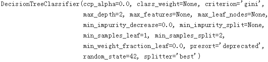
iris.keys()![]()
You can visualize the trained Decision Tree by first using the export_graphviz() method to output a graph definition file called iris_tree.dot:
# pip3 install graphviz
from graphviz import Source
from sklearn.tree import export_graphviz
import os
os.environ["PATH"] += os.pathsep + "D:/Graphviz2.38/bin" # " directory" where you intall graphviz

export_graphviz(
    tree_clf,
    out_file = os.path.join( "iris_tree.dot"),
    feature_names = iris.feature_names[2:], ###
    class_names = iris.target_names,###
    rounded = True,
    filled = True
)

Source.from_file("iris_tree.dot")
Figure 6-1. Iris Decision Tree
#########################################################################
https://blog.csdn.net/Linli522362242/article/details/104124771
Gini impurity
Used by the CART (Classification And Regression Tree) algorithm for classification trees, Gini impurity is a measure of how often a randomly chosen element from the set would be incorrectly labeled if it was randomly labeled according to the distribution of labels in the subset. The Gini impurity can be computed by summing the probability ![]() of an item with label i being chosen times the probability
of an item with label i being chosen times the probability ![]() of a mistake in categorizing that item. It reaches its minimum (zero) when all cases in the node fall into a single target category.
of a mistake in categorizing that item. It reaches its minimum (zero) when all cases in the node fall into a single target category.
To compute Gini impurity for a set of items with ![]() classes, suppose
classes, suppose ![]() , and let
, and let ![]() be the fraction of items labeled with class
be the fraction of items labeled with class ![]() in the set. (
in the set. (![]() is the proportion of class i in the set)
is the proportion of class i in the set) 
![]()
![]() : the sum of all probabilities of all classes(J) is equal to 1.
: the sum of all probabilities of all classes(J) is equal to 1.

example: 
![]() and 1 ==
and 1 == ![]() +
+ ![]() +
+ ![]()
#########################################################################
Making Predictions
Let’s see how the tree represented in Figure 6-1 makes predictions. Suppose you find an iris flower and you want to classify it. You start at the root node (depth 0, at the top): this node asks whether the flower’s petal length is smaller than 2.45 cm. If it is, then you move down to the root’s left child node (depth 1, left). In this case, it is a leaf node (i.e., it does not have any children nodes), so it does not ask any questions: you can simply look at the predicted class for that node and the Decision Tree predicts that your flower is an Iris-Setosa (class=setosa).
Now suppose you find another flower, but this time the petal length is greater than 2.45 cm. You must move down to the root’s right child node (depth 1, right), which is not a leaf node, so it asks another question: is the petal width smaller than 1.75 cm? If it is, then your flower is most likely an Iris-Versicolor (depth 2, left). If not, it is likely an Iris-Virginica (depth 2, right). It’s really that simple. (see following: Prediction via Stratification of the Feature Space)
#################################
NOTE
One of the many qualities of Decision Trees is that they require very little data preparation. In particular, they don’t require feature scaling or centering at all.
#################################
A node’s samples attribute counts how many training instances it applies to. For example, 100 training instances have a petal width greater than 2.45 cm (depth 1, right), among which 54 have a petal width smaller than 1.75 cm (depth 2, left). A node’s value attribute tells you how many training instances of each class this node applies to: for example, the bottom-right node applies to 0 Iris-Setosa, 1 Iris-Versicolor, and 45 Iris-Virginica. Finally, a node’s gini attribute measures its impurity不纯: a node is “pure” (gini=0) if all training instances it applies to belong to the same class. For example, since the depth-1 left node applies only to Iris-Setosa training instances, it is pure and its gini score is 0. Equation 6-1 shows how the training algorithm computes the gini score ![]() of the ith node. For example, the depth-2 left node has a gini score equal to
of the ith node. For example, the depth-2 left node has a gini score equal to ![]() . Another impurity measure is discussed shortly.
. Another impurity measure is discussed shortly.
Equation 6-1. Gini impurity![]()
![]() is the ratio of class k instances among the training instances in the
is the ratio of class k instances among the training instances in the ![]() node/region.
node/region.

#################################
NOTE
Scikit-Learn uses the CART algorithm, which produces only binary trees: nonleaf nodes always have two children (i.e., questions only have yes/no answers). However, other algorithms such as ID3 can produce Decision Trees with nodes that have more than two children.
#################################
from matplotlib.colors import ListedColormap
%matplotlib inline
import matplotlib as mpl
import matplotlib.pyplot as plt

def plot_decision_boundary(clf, X, y, axes=[0, 7.5, 0, 3], iris=True, legend=False, plot_training=True):
    x1s = np.linspace( axes[0], axes[1], 100 )
    x2s = np.linspace( axes[2], axes[3], 100 )
    x1, x2 = np.meshgrid( x1s, x2s )
    X_new = np.c_[ x1.ravel(), x2.ravel() ]
    y_pred = clf.predict( X_new ).reshape( x1.shape )
    print("Classified y_pred:",np.unique(y_pred)) #Classified y_pred: [0 1 2]
    custom_cmap = ListedColormap(['#fafab0','#9898ff','r']) #since y_pred
    plt.contourf( x1, x2, y_pred, alpha=0.3, cmap=custom_cmap )
#     if not iris:
#         custom_cmap2 = ListedColormap(['#7d7d58','#4c4c7f','#507d50'])
#         plt.contour( x1, x2, y_pred, cmap=custom_cmap2, alpha=0.8 )
    if plot_training:
        plt.plot( X[:,0][y==0], X[:,1][y==0], "yo", label="Iris setosa" )
        plt.plot( X[:,0][y==1], X[:,1][y==1], "bs", label="Iris versicolor")
        plt.plot( X[:,0][y==2], X[:,1][y==2], "g^", label="Iris virginica")
        plt.axis(axes)
    if iris:
        plt.xlabel( "Petal length", fontsize=14 )
        plt.ylabel( "Petal width", fontsize=14 )
    else:
        plt.xlabel( r"$x_1$", fontsize=18 )
        plt.ylabel( r"$x_2$", fontsize=18, rotation=0 )
#     if legend:
#         plt.legend( loc="lower right", fontsize=14 )

plt.figure( figsize=(8,4) )
plot_decision_boundary( tree_clf, X,y )
          # petal length (cm) <=2.45
plt.plot( [2.45, 2.45], [0, 3], "k-", linewidth=2 ) # Depth=0
                       # petal width (cm) <= 1.75
plt.plot( [2.45, 7.5], [1.75, 1.75], "k--", linewidth=2) # Depth=1
plt.plot( [4.95, 4.95], [0, 1.75], "k:", linewidth=2) # Depth=2
plt.plot( [4.85, 4.85], [1.75, 3], "k:", linewidth=2)

plt.text(1.3, 1.0, "Depth=0", fontsize=15)
plt.text(3.2, 1.8, "Depth=1", fontsize=13)
plt.text(4.0, 0.5, "(Depth=2)", fontsize=11)

plt.show()
Classified y_pred: [0 1 2]
Figure 6-2. Decision Tree decision boundaries
Figure 6-2 shows this Decision Tree’s decision boundaries. The thick vertical line represents the decision boundary of the root node (depth 0): petal length = 2.45 cm. Since the left area is pure (only Iris-Setosa), it cannot be split any further. However, the right area is impure, so the depth-1 right node splits it at petal width = 1.75 cm (represented by the dashed line). Since max_depth was set to 2, the Decision Tree stops right there.
################################################extra materials
Decision trees can be applied to both regression and classification problems. We first consider regression problems, and then move on to classification.
FIGURE 8.1. For the Hitters data, a regression tree for predicting the log salary of a baseball player, based on the number of years that he has played in the major leagues大联盟 and the number of hits that he made in the previous year. At a given internal node, the label (of the form ![]() ) indicates the left-hand branch emanating from that split, and the right-hand branch corresponds to
) indicates the left-hand branch emanating from that split, and the right-hand branch corresponds to ![]() . For instance, the split at the top of the tree results in two large branches. The left-hand branch corresponds to Years<4.5, and the right-hand branch corresponds to Years>=4.5. The tree has two internal nodes and three terminal nodes, or leaves. The number in each leaf is the mean of the response for the observations that fall there.
. For instance, the split at the top of the tree results in two large branches. The left-hand branch corresponds to Years<4.5, and the right-hand branch corresponds to Years>=4.5. The tree has two internal nodes and three terminal nodes, or leaves. The number in each leaf is the mean of the response for the observations that fall there.
8.1.1 Regression Trees
In order to motivate regression trees, we begin with a simple example.
Predicting Baseball Players’Salaries Using Regression Trees
We use the Hitters data set to predict a baseball player's Salary based on Years (the number of years that he has played in the major leagues) and Hits (the number of hits that he made in the previous year).We first remove observations that are missing Salary values, and log-transform Salary so that its distribution has more of a typical bell-shape. (Recall that Salary is measured in thousands of dollars.)
Figure 8.1 shows a regression tree fit to this data. It consists of a series of splitting rules, starting at the top of the tree. The top split assigns observations having Years<4.5 to the left branch. The predicted salary for these players is given by the mean (or average)response value for the players in the data set with Years<4.5. For such players, the mean (or average) log salary is 5.107(or 5.11), and so we make a prediction of ![]() thousands of dollars, i.e. $165,174, for these players. Players with Years>=4.5 are assigned to the right branch, and then that group is further subdivided by Hits. Overall, the tree stratifies or segments the players into three regions of predictor space: players who have played for four or fewer years R1 ={X | Years<4.5}, players who have played for five or more years and who made fewer than 118 hits last year R2 ={X | Years>=4.5, Hits<117.5}, and players who have played for five or more years and who made at least 118 hits last year R3 ={X | Years>=4.5, Hits>=117.5}. Figure 8.2 illustrates the regions as a function of Years and Hits. The predicted salaries for these three groups are $1,000×
thousands of dollars, i.e. $165,174, for these players. Players with Years>=4.5 are assigned to the right branch, and then that group is further subdivided by Hits. Overall, the tree stratifies or segments the players into three regions of predictor space: players who have played for four or fewer years R1 ={X | Years<4.5}, players who have played for five or more years and who made fewer than 118 hits last year R2 ={X | Years>=4.5, Hits<117.5}, and players who have played for five or more years and who made at least 118 hits last year R3 ={X | Years>=4.5, Hits>=117.5}. Figure 8.2 illustrates the regions as a function of Years and Hits. The predicted salaries for these three groups are $1,000×![]() =$165,174 (log salary is 5.107 or 5.11), $1,000×
=$165,174 (log salary is 5.107 or 5.11), $1,000×![]() =$402,834 (log salary is 5.999 or 6.00), and $1,000×
=$402,834 (log salary is 5.999 or 6.00), and $1,000×![]() =$845,346 (log salary is 6.74) respectively.
=$845,346 (log salary is 6.74) respectively.

FIGURE 8.2. The three-region partition for the Hitters data set from the regression tree illustrated in Figure 8.1.
In keeping with the tree analogy, the regions R1, R2, and R3 are known as terminal nodes or leaves of the tree. As is the case for Figure 8.1, decision terminal node leaf trees are typically drawn upside down, in the sense that the leaves are at the bottom of the tree. The points along the tree where the predictor space(预测变最空间) is split are referred to as internal nodes. In Figure 8.1, the two internal internal node nodes are indicated by the text Years<4.5 and Hits<117.5. We refer to the segments of the trees that connect the nodes as branches.
We might interpret the regression tree displayed in Figure 8.1 as follows: Years is the most important factor in determining Salary, and players with less experience earn lower salaries than more experienced players. Given that a player is less experienced, the number of hits that he made in the previous year seems to play little role in his salary. But among players who have been in the major leagues for five or more years, the number of hits made in the previous year does affect salary, and players who made more hits last year tend to have higher salaries. The regression tree shown in Figure 8.1 is likely an over-simplification of the true relationship between Hits, Years, and Salary. However, it has advantages over other types of regression models (such as those seen in Chapters 3 and 6): it is easier to interpret, and has a nice graphical representation.
Prediction via Stratification of the Feature Space
We now discuss the process of building a regression tree. Roughly speaking, there are two steps.
- We divide the predictor space(预测变量空间) —that is, the set of possible values for
 —into J distinct and non-overlapping regions,
  . (used predictor/selected feature to split the dataset), for example Years<4.5, Years is a predictor)
 - For every observation that falls into the region
 , we make the same prediction, which is simply the mean(or average) of the response values for the training observations in
  .
.
For instance, suppose that in Step 1 we obtain two regions, R1 and R2, and that the response mean(or average) of the training observations in the first region is 10, while the response mean(or average) of the training observations in the second region is 20. Then for a given observation X = x, if x ∈ R1 we will predict a value of 10, and if x ∈ R2 we will predict a value of 20.
We now elaborate详尽说明 on Step 1 above. How do we construct the regions ![]() ? In theory, the regions could have any shape. However, we choose to divide the predictor space into high-dimensional rectangles, or boxes, for simplicity and for ease of interpretation of the resulting predictive model. The goal is to find boxes
? In theory, the regions could have any shape. However, we choose to divide the predictor space into high-dimensional rectangles, or boxes, for simplicity and for ease of interpretation of the resulting predictive model. The goal is to find boxes ![]() that minimize the RSS(Residuals Sum of Squared), given by
that minimize the RSS(Residuals Sum of Squared), given by where
where ![]() is the mean(or average) response for the training observations within the
is the mean(or average) response for the training observations within the ![]() box. (yi
box. (yi ![]() is Actual True Target Value )Unfortunately, it is computationally infeasible不可实行的 to consider every possible partition of the feature space into J boxes. For this reason, we take a top-down自上而下, 贪婪greedy approach that is known as recursive binary splitting递归二叉分裂. The recursive binary splitting approach is top-down because it begins at the top of the tree (at which point all observations belong to a single region) and then successively splits the predictor space; each split is indicated via two new branches further down on the tree. It is greedy because at each step of the tree-building process, the best split is made at that particular step, rather than looking ahead and picking a split that will lead to a better tree in some future step.
is Actual True Target Value )Unfortunately, it is computationally infeasible不可实行的 to consider every possible partition of the feature space into J boxes. For this reason, we take a top-down自上而下, 贪婪greedy approach that is known as recursive binary splitting递归二叉分裂. The recursive binary splitting approach is top-down because it begins at the top of the tree (at which point all observations belong to a single region) and then successively splits the predictor space; each split is indicated via two new branches further down on the tree. It is greedy because at each step of the tree-building process, the best split is made at that particular step, rather than looking ahead and picking a split that will lead to a better tree in some future step.
In order to perform recursive binary splitting, we first select the predictor ![]() (from
(from ![]() ) and the cutpoint分割点 s such that splitting the predictor space into the regions {X|
) and the cutpoint分割点 s such that splitting the predictor space into the regions {X|![]() < s} and {X|
< s} and {X|![]() ≥ s} leads to the greatest possible reduction in RSS. (The notation {X|
≥ s} leads to the greatest possible reduction in RSS. (The notation {X|![]() < s} means the region of predictor space in which
< s} means the region of predictor space in which ![]() takes on a value less than s.) That is, we consider all predictors
takes on a value less than s.) That is, we consider all predictors ![]() , and all possible values of the cutpoint s for each of the predictors, and then choose the predictor and cutpoint such that the resulting tree has the lowest RSS. In greater detail, for any j and cutpoint s, we
, and all possible values of the cutpoint s for each of the predictors, and then choose the predictor and cutpoint such that the resulting tree has the lowest RSS. In greater detail, for any j and cutpoint s, we
define the pair of half-planes ![]()
and we seek the value of j and s that minimize the equation

where ![]() is the mean response for the training observations in
is the mean response for the training observations in ![]() , and
, and ![]() is the mean response for the training observations in
is the mean response for the training observations in ![]() . Finding the values of j (or the predictor
. Finding the values of j (or the predictor ![]() )and s that minimize (8.3) can be done quite quickly, especially when the number of features p is not too large.
)and s that minimize (8.3) can be done quite quickly, especially when the number of features p is not too large.
Next, we repeat the process, looking for the best predictor and best cutpoint in order to split the data further so as to minimize the RSS within each of the resulting regions. However, this time, instead of splitting the entire predictor space, we split one of the two previously identified regions. We now have three regions. Again, we look to split one of these three regions further, so as to minimize the RSS. The process continues until a stopping criterion is reached; for instance, we may continue until no region contains more than five observations.
Once the regions ![]() have been created, we predict the response for a given test observation using the mean of the training observations in the region to which that test observation belongs.
have been created, we predict the response for a given test observation using the mean of the training observations in the region to which that test observation belongs.
A five-region example of this approach is shown in Figure 8.3.
 FIGURE 8.3. Top Left: A partition of two-dimensional feature space that could not result from recursive binary splitting. Top Right: The output of recursive binary splitting on a two-dimensional example. Bottom Left: A tree corresponding to the partition in the top right panel. Bottom Right: A perspective plot of the prediction surface corresponding to that tree.
################################################
However, if you set max_depth to 3, then the two depth-2 nodes would each add another decision boundary (represented by the dotted lines).
###############################################################
Model Interpretation: White Box Versus Black Box
As you can see Decision Trees are fairly intuitive and their decisions are easy to interpret.
Such models are often called white box models. In contrast, as we will see, Random Forests or neural networks are generally considered black box models. They make great predictions, and you can easily check the calculations that they performed to make these predictions; nevertheless, it is usually hard to explain in simple terms why the predictions were made. For example, if a neural network says that a particular person appears on a picture, it is hard to know what actually contributed to导致 this prediction: did the model recognize that person’s eyes? Her mouth? Her nose? Her shoes? Or even the couch that she was sitting on? Conversely, Decision Trees provide nice and simple classification rules that can even be applied manually if need be (e.g., for flower classification).
###############################################################
Estimating Class Probabilities
A Decision Tree can also estimate the probability that an instance belongs to a particular class k: first it traverses the tree to find the leaf node for this instance, and then it returns the ratio of training instances of class k in this node. For example, suppose you have found a flower whose petals are 5 cm long and 1.5 cm wide. The corresponding leaf node is the depth-2 left node, so the Decision Tree should output the following probabilities: 0% for Iris-Setosa (0/54), 90.7% for Iris-Versicolor (49/54), and 9.3% for Iris-Virginica (5/54). And of course if you ask it to predict the class, it should output Iris-Versicolor (class 1) since it has the highest probability. Let’s check this:
tree_clf.predict_proba([ [5, 1.5] ])![]()
tree_clf.predict([ [5, 1.5] ])![]()
iris.target_names[ tree_clf.predict([ [5, 1.5] ]) ]![]()
Perfect! Notice that the estimated probabilities would be identical anywhere else in the bottom-right rectangle of Figure 6-2—for example, if the petals were 6 cm long and 1.5 cm wide (even though it seems obvious that it would most likely be an Iris-Virginica![]() in this case).
in this case).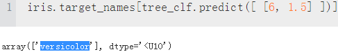

The CART Training Algorithm
Scikit-Learn uses the Classification And Regression Tree (CART) algorithm to train Decision Trees (also called “growing” trees). The idea is really quite simple: the algorithm first splits the training set in two subsets using a single feature k and a threshold ![]() (e.g., “petal length ≤ 2.45 cm”). How does it choose k and
(e.g., “petal length ≤ 2.45 cm”). How does it choose k and ![]() ? It searches for the pair (k,
? It searches for the pair (k, ![]() ) that produces the purest subsets (weighted by their size). The cost function that the algorithm tries to minimize is given by Equation 6-2.
) that produces the purest subsets (weighted by their size). The cost function that the algorithm tries to minimize is given by Equation 6-2.
Equation 6-2. CART cost function for classification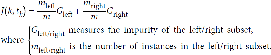
Once it has successfully split the training set in two, it splits the subsets using the same logic, then the sub-subsets and so on, recursively. It stops recursing once it reaches the maximum depth (defined by the max_depth hyperparameter), or if it cannot find a split that will reduce impurity. A few other hyperparameters (described in a moment) control additional stopping conditions (min_samples_split, min_samples_leaf, min_weight_fraction_leaf, and max_leaf_nodes).
###############################################
WARNING
As you can see, the CART algorithm is a greedy贪婪 algorithm: it greedily searches for an optimum split at the top level, then repeats the process at each level. It does not check whether or not the split will lead to the lowest possible impurity several levels down. A greedy algorithm often produces a reasonably good solution, but it is not guaranteed to be the optimal solution.
###############################################
Unfortunately, finding the optimal tree is known to be an NP-Complete problem: it requires ![]() time, making the problem intractable难对付的 even for fairly small training sets. This is why we must settle解决 for a “reasonably good”(而不是最佳的) solution.
time, making the problem intractable难对付的 even for fairly small training sets. This is why we must settle解决 for a “reasonably good”(而不是最佳的) solution.
Computational Complexity
Making predictions requires traversing the Decision Tree from the root to a leaf. Decision Trees are generally approximately balanced, so traversing the Decision Tree requires going through roughly ![]() nodes(log2 is the binary logarithm. It is equal to
nodes(log2 is the binary logarithm. It is equal to ![]() = log(m) / log(2).). Since each node(in n) only requires checking the value of one feature, the overall prediction complexity is just
= log(m) / log(2).). Since each node(in n) only requires checking the value of one feature, the overall prediction complexity is just ![]() , independent of the number of features与特征的数量无关. So predictions are very fast, even when dealing with large training sets.
, independent of the number of features与特征的数量无关. So predictions are very fast, even when dealing with large training sets.
However, the training algorithm compares all features (or less if max_features is set) on all samples at each node. This results in a training complexity训练时间复杂度 of ![]() (n-dimensions OR n-features, m numbers of instances). For small training sets (less than a few thousand instances), Scikit-Learn can speed up training by presorting the data (set presort=True), but this slows down training considerably for larger training sets.
(n-dimensions OR n-features, m numbers of instances). For small training sets (less than a few thousand instances), Scikit-Learn can speed up training by presorting the data (set presort=True), but this slows down training considerably for larger training sets.
Gini Impurity or Entropy?
By default, the Gini impurity measure is used, but you can select the entropy impurity measure instead by setting the criterion标准 hyperparameter to "entropy". The concept of entropy originated in thermodynamics热力学 as a measure of molecular分子 disorder: entropy熵 approaches zero when molecules are still and well ordered当分子井然有序的时候,熵值接近于 0. It later spread to a wide variety of domains, including Shannon's information theory, where it measures the average information content of a message: entropy is zero when all messages are identical. In Machine Learning, it is frequently used as an impurity measure: a set's entropy is zero when it contains instances of only one class. Equation 6-3 shows the definition of the entropy of the ith node. For example, the depth-2 left node in Figure 6-1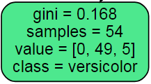 has an entropy equal to
 ![]() .
.
Equation 6-3. Entropy
So should you use Gini impurity or entropy? The truth is, most of the time it does not make a big difference: they lead to similar trees. Gini impurity is slightly faster to compute, so it is a good default. However, when they differ, Gini impurity tends to isolate the most frequent class in its own branch of the tree, while entropy tends to produce slightly more balanced trees.
Regularization Hyperparameters正则化超参数
Decision Trees make very few assumptions about the training data (as opposed to linear models, which obviously assume that the data is linear, for example). If left unconstrained如果不添加约束, the tree structure will adapt itself to the training data, fitting it very closely, and most likely overfitting it. Such a model is often called a nonparametric model, not because it does not have any parameters (it often has a lot) but because the number of parameters is not determined prior to training, so the model structure is free to stick closely to the data所以模型结构可以根据数据的特性自由生长.
In contrast, a parametric model such as a linear model has a predetermined number of parameters, so its degree of freedom is limited, reducing the risk of overfitting (but increasing the risk of underfitting).
To avoid overfitting the training data, you need to restrict the Decision Tree's freedom during training. As you know by now, this is called regularization. The regularization hyperparameters depend on the algorithm used, but generally you can at least restrict the maximum depth of the Decision Tree. In Scikit-Learn, this is controlled by the max_depth hyperparameter (the default value is None, which means unlimited). Reducing max_depth will regularize the model and thus reduce the risk of overfitting.(see following: Tree Pruning 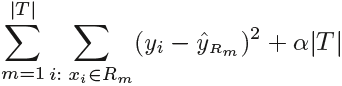 )
)
The DecisionTreeClassifier class has a few other parameters that similarly restrict the shape of the Decision Tree: min_samples_split (the minimum number of samples a node must have before it can be split), min_samples_leaf (the minimum number of samples a leaf node must have), min_weight_fraction_leaf (same as min_samples_leaf but expressed as a fraction of the total number of weighted instances), max_leaf_nodes (maximum number of leaf nodes), and max_features (maximum number of features that are evaluated for splitting at each node). Increasing min_* hyperparameters or reducing max_* hyperparameters will regularize the model.
#########################################
NOTE
Other algorithms work by first training the Decision Tree without restrictions, then pruning剪枝 (deleting) unnecessary nodes. A node whose children are all leaf nodes is considered unnecessary( if the purity improvement it provides is not statistically significant).
Standard statistical tests, such as the χ2 test, are used to estimate the probability that the improvement is purely the result of chance改进是否纯粹是偶然性的结果 (which is called the null hypothesis). If this probability, called the p-value, is higher than a given threshold (typically 5%, controlled by a hyperparameter也就是 95% 置信度), then the node is considered unnecessary and its children are deleted. The pruning continues until all unnecessary nodes have been pruned.
#########################################
Figure 6-3 shows two Decision Trees trained on the moons dataset (introduced in https://blog.csdn.net/Linli522362242/article/details/104280075). On the left, the Decision Tree is trained with the default hyperparameters (i.e., no restrictions), and on the right the Decision Tree is trained with min_samples_leaf=4. It is quite obvious that the model on the left is overfitting, and the model on the right will probably generalize better.
from sklearn.datasets import make_moons
Xm, ym = make_moons( n_samples=100, noise=0.25, random_state=53 )#X[:, x1 or x2], y[0 or 1]

deep_tree_clf1 = DecisionTreeClassifier( random_state=42 )#with the default hyperparameters
deep_tree_clf2 = DecisionTreeClassifier( min_samples_leaf=4, random_state=42 )
deep_tree_clf1.fit(Xm, ym)
deep_tree_clf2.fit(Xm, ym)

from matplotlib.colors import ListedColormap
%matplotlib inline
import matplotlib as mpl
import matplotlib.pyplot as plt

def plot_decision_boundary(clf, X, y, axes=[0, 7.5, 0, 3], iris=True, legend=False, plot_training=True):
    x1s = np.linspace( axes[0], axes[1], 100 )
    x2s = np.linspace( axes[2], axes[3], 100 )
    x1, x2 = np.meshgrid( x1s, x2s )
    X_new = np.c_[ x1.ravel(), x2.ravel() ]
    y_pred = clf.predict( X_new ).reshape( x1.shape )
    custom_cmap = ListedColormap(['#fafab0','#9898ff','#a0faa0'])
    plt.contourf( x1, x2, y_pred, alpha=0.3, cmap=custom_cmap )############

    if not iris:
        custom_cmap2 = ListedColormap(['#7d7d58','#4c4c7f','#507d50'])
        plt.contour( x1, x2, y_pred, cmap=custom_cmap2, alpha=0.8 )
    if plot_training:
        plt.plot( X[:,0][y==0], X[:,1][y==0], "yo", label="Iris setosa" )
        plt.plot( X[:,0][y==1], X[:,1][y==1], "bs", label="Iris versicolor")
        plt.plot( X[:,0][y==2], X[:,1][y==2], "g^", label="Iris virginica")
        plt.axis(axes)
    if iris:
        plt.xlabel( "Petal length", fontsize=14 )
        plt.ylabel( "Petal width", fontsize=14 )
    else:
        plt.xlabel( r"$x_1$", fontsize=18 )
        plt.ylabel( r"$x_2$", fontsize=18, rotation=0 )
    if legend:
        plt.legend( loc="lower right", fontsize=14 )

fig, axes = plt.subplots( ncols=2, figsize=(16,4), sharey=True )

plt.sca( axes[0] )
plot_decision_boundary( deep_tree_clf1, Xm, ym, axes=[-1.5, 2.4, -1, 1.5], iris=False )
plt.title( "No restrictions", fontsize=16 )

plt.sca( axes[1] )
plot_decision_boundary( deep_tree_clf2, Xm, ym, axes=[-1.5, 2.4, -1, 1.5], iris=False )
plt.title( "min_samples_leaf = {}".format(deep_tree_clf2.min_samples_leaf), fontsize=14 )
plt.ylabel("") #remove the ylabel

plt.show()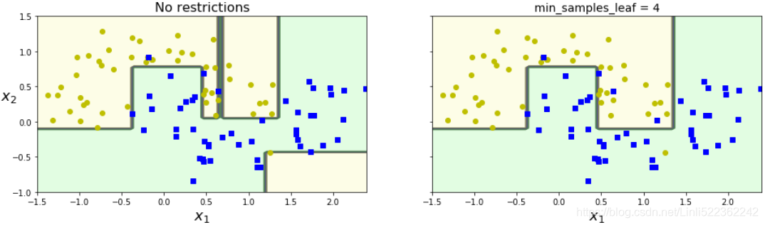
Figure 6-3. Regularization using min_samples_leaf(叶节点必须具有的最小样本数)
Regression
Decision Trees are also capable of performing regression tasks. Let's build a regression tree using Scikit-Learn’s DecisionTreeRegressor class, training it on a noisy quadratic dataset with max_depth=2:
# Quadratic training set + noise
np.random.seed(42)
m=200
X = np.random.rand(m,1)
y = 4 * (X-0.5)**2 + np.random.randn(m,1) / 10 # +noise

from sklearn.tree import DecisionTreeRegressor

tree_reg = DecisionTreeRegressor(max_depth=2, random_state=42)
tree_reg.fit(X,y) 
# pip3 install graphviz
from graphviz import Source
from sklearn.tree import export_graphviz
import os

os.environ["PATH"] += os.pathsep + "D:/Graphviz2.38/bin" # " directory" where you intall graphviz

export_graphviz(
    tree_reg1,
    out_file = os.path.join("regression_tree.dot"),
    feature_names = ["x1"], ###
    rounded = True,
    filled = True
)

Source.from_file("regression_tree.dot")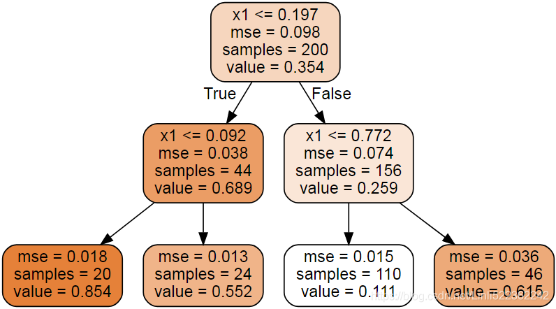
Figure 6-4. A Decision Tree for regression
This tree looks very similar to the classification tree you built earlier. The main difference is that instead of predicting a class in each node, it predicts a value. For example, suppose you want to make a prediction for a new instance with x1 = 0.6. You traverse the tree starting at the root, and you eventually reach the leaf node that predicts value=0.111. This prediction is simply the average target value of the 110 training instances associated to this leaf node. This prediction results in a Mean Squared Error (MSE) equal to 0.015 over these 110 instances.
from sklearn.tree import DecisionTreeRegressor

tree_reg1 = DecisionTreeRegressor(random_state=42, max_depth=2)
tree_reg2 = DecisionTreeRegressor(random_state=42, max_depth=3)
tree_reg1.fit(X,y)
tree_reg2.fit(X,y)

def plot_regression_predictions( tree_reg, X,y, axes=[0,1, -0.2,1], ylabel="$y$" ):
    x1 = np.linspace( axes[0], axes[1], 500).reshape(-1,1)
    y_pred = tree_reg.predict(x1)
    plt.axis(axes)
    plt.xlabel( "$x_1$", fontsize=18, rotation=0 )
    if ylabel:
        plt.ylabel(ylabel, fontsize=18, rotation=0)

    plt.plot( X, y, "b." )
    #the predicted value for each region is always the average target value of the
    #instances in that region
    plt.plot( x1,y_pred, 'r.-', linewidth=2, label=r"$\hat{y}$" )

fig, axes = plt.subplots(ncols=2, figsize=(10,4), sharey=True)

plt.sca( axes[0] )
plot_regression_predictions(tree_reg1, X,y)
                       #depth=1       #depth=2         #depth=2
for split, style in ( (0.1973, "y-"), (0.0917, "y--"), (0.7718,"y--") ):
    plt.plot( [split, split], [-0.2,1], style, linewidth=2 ) # splitting lines
plt.text(0.21, 0.65, "Depth=0", fontsize=15)
plt.text(0.01, 0.2,  "Depth=1", fontsize=13)
plt.text(0.65, 0.8,  "Depth=1", fontsize=13)
plt.legend(loc="upper center", fontsize=18)
plt.title("max_depth=2", fontsize=14)

plt.sca( axes[1] )
plot_regression_predictions(tree_reg2, X,y, ylabel=None)
                      #depth=1        #depth=2         #depth=2
for split, style in ( (0.1973, "y-"), (0.0917, "y--"), (0.7718,"y--") ):
    plt.plot( [split, split], [-0.2,1], style, linewidth=2 )# splitting line
for split in (0.0458, 0.1298, 0.2873, 0.9040): #depth=3
    plt.plot( [split, split], [-0.2,1], "k:", linewidth=1 ) # splitting lines
plt.text(0.3, 0.5, "Depth=2", fontsize=14)
plt.title("max_depth=3", fontsize=14)

plt.show()
Figure 6-5. Predictions of two Decision Tree regression models
注:图里面的红线就是训练实例的平均目标值,对应上图中的 the predicted value of the instances in that region
This model's predictions are represented on the left of Figure 6-5. If you set max_depth=3, you get the predictions represented on the right. Notice how the predicted value for each region is always the average target value of the instances in that region. The algorithm splits each region in a way that makes most training instances as close as possible to that predicted value. 算法以一种使大多数训练实例尽可能接近该预测值的方式分割每个区域。
The CART algorithm works mostly the same way as earlier, except that instead of trying to split the training set in a way that minimizes impurity, it now tries to split the training set in a way that minimizes the MSE. Equation 6-4 shows the cost function that the algorithm tries to minimize.
Equation 6-4. CART cost function for regression
Just like for classification tasks, Decision Trees are prone to overfitting when dealing with regression tasks. Without any regularization (i.e., using the default hyperparameters), you get the predictions on the left of Figure 6-6. It is obviously overfitting the training set very badly. Just setting min_samples_leaf=10 results in a much more reasonable model, represented on the right of Figure 6-6.
tree_reg1 = DecisionTreeRegressor(random_state=42) #Without any regularization and using the default hyperparameters
tree_reg2 = DecisionTreeRegressor(random_state=42, min_samples_leaf = 10)
tree_reg1.fit(X,y)
tree_reg2.fit(X,y)

x1 = np.linspace(0,1, 500).reshape(-1,1)
y_pred1 = tree_reg1.predict(x1)
y_pred2 = tree_reg2.predict(x1)

fig, axes = plt.subplots(ncols=2, figsize=(10,4), sharey=True)

plt.sca(axes[0])
plt.plot(X,  y, "b.")
plt.plot(x1, y_pred1, "r.-", linewidth=2, label=r"$\hat {y}$" )
plt.axis([0,1,-0.2, 1.1])
plt.xlabel("$x_1$", fontsize=18)
plt.ylabel("$y$", fontsize=18, rotation=0)
plt.legend(loc="upper center", fontsize=18)
plt.title("No restrictions", fontsize=14)

plt.sca(axes[1])
plt.plot(X, y, "b.")
plt.plot(x1, y_pred2, "r.-", linewidth=2, label=r"$\hat {y}$" )
plt.axis([0,1,-0.2,1.1])
plt.xlabel("$x_1$", fontsize=18)
plt.title("min_samples_leaf={}".format(tree_reg2.min_samples_leaf), fontsize=14)

plt.show()
Figure 6-6. Regularizing a Decision Tree regressor
You get the predictions on the left of Figure 6-6. It is obviously overfitting the training set very badly. Just setting min_samples_leaf=10 results in a much more reasonable model, represented on the right of Figure 6-6
Instability(Decision Trees are very sensitive to small variations变化 in the training data)
Hopefully by now you are convinced that Decision Trees have a lot going for them: they are simple to understand and interpret, easy to use, versatile多用途的, and powerful. However they do have a few limitations. First, as you may have noticed, Decision
Trees love orthogonal正交化 decision boundaries (all splits are perpendicular to an axis), which makes them sensitive to training set rotation. For example, Figure 6-7 shows a simple linearly separable dataset: on the left, a Decision Tree can split it easily, while on the right, after the dataset is rotated by 45°, the decision boundary looks unnecessarily convoluted卷曲的/复杂的. Although both Decision Trees fit the training set perfectly, it is very likely that the model on the right will not generalize well. One way to limit this problem is to use PCA, which often results in a better orientation of the training data.
np.random.seed(6)
Xs = np.random.rand(100,2)-0.5# between [0, 1)-0.5
                   #True/False-->1/0 then times 2 == 2/0
ys = (Xs[:, 0] > 0).astype(np.float32) * 2

Xs[:5]
angle = np.pi/4  #rotaion angle
rotation_maxtrix = np.array([ [np.cos(angle), -np.sin(angle)], [np.sin(angle), np.cos(angle)] ])
Xsr = Xs.dot( rotation_maxtrix)
Xsr[:5]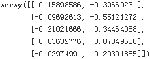
tree_clf_s = DecisionTreeClassifier( random_state=42 )
tree_clf_s.fit( Xs,ys )

tree_clf_sr = DecisionTreeClassifier( random_state=42 )
tree_clf_sr.fit( Xsr,ys )

fig, axes = plt.subplots( ncols=2, figsize=(10,4), sharey=True )

plt.sca( axes[0] )
plot_decision_boundary( tree_clf_s, Xs, ys, axes=[-0.7,0.7, -0.7,0.7], iris=False )

plt.sca( axes[1] )
plot_decision_boundary( tree_clf_sr, Xsr, ys, axes=[-0.7,0.7, -0.7,0.7], iris=False)
plt.ylabel("")

plt.subplots_adjust(wspace=0.05)
plt.title("Figure 6-7. Sensitivity to training set rotation")
plt.show()
Figure 6-7. Sensitivity to training set rotation
on the left, a Decision Tree can split it easily, while on the right, after the dataset is rotated by 45°, the decision boundary looks unnecessarily convoluted卷曲的/复杂的. Although both Decision Trees fit the training set perfectly, it is very likely that the model on the right will not generalize well.
iris = load_iris()
X = iris.data[:, 2:] # petal length and width
y = iris.target

angle = np.pi / 180 * 20
rotation_matrix = np.array([[np.cos(angle), -np.sin(angle)], [np.sin(angle), np.cos(angle)]])
Xr = X.dot(rotation_matrix)

tree_clf_r = DecisionTreeClassifier(random_state=42)
tree_clf_r.fit(Xr, y)

plt.figure(figsize=(8, 3))
plot_decision_boundary(tree_clf_r, Xr, y, axes=[0.5, 7.5, -1.0, 1], iris=False)

plt.show()
More generally, the main issue with Decision Trees is that they are very sensitive to small variations变化 in the training data. For example, if you just remove the widest Iris-Versicolor from the iris training set (the one with petals 4.8 cm long and 1.8 cm wide) and train a new Decision Tree, you may get the model represented in Figure 6-8. As you can see, it looks very different from the previous Decision Tree (Figure 6-2). Actually, since the training algorithm used by Scikit-Learn is stochastic you may get very different models even on the same training data (unless you set the random_state hyperparameter).
      # X[:,1][y==1].max() get the Iris versicolor's the largeist width
X[ ( X[:, 1]== X[:,1][y==1].max() )&(y==1) ] # the widest Iris versicolor((y==1)) flower's attributes value![]()
not_widest_versicolor = (X[:,1]!=1.8) | (y==2) #Iris' width !=1.8 for ignoring the widest Versicolor or Virginica(y==2)
X_tweaked = X[not_widest_versicolor]
y_tweaked = y[not_widest_versicolor]

tree_clf_tweaked = DecisionTreeClassifier( max_depth=2, random_state=40 )
tree_clf_tweaked.fit(X_tweaked, y_tweaked)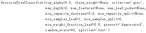
plt.figure( figsize=(8,4) )
plot_decision_boundary( tree_clf_tweaked, X_tweaked, y_tweaked, legend=False)
plt.plot( [0,7.5], [0.8,0.8], 'k-', linewidth=2 )
plt.plot( [0,7.5], [1.75,1.75], 'k--', linewidth=2 )
plt.text(1.0,0.9, "Depth=0", fontsize=15)
plt.text(1.0,1.8, "Depth=1", fontsize=13)

plt.show()
Figure 6-8. Sensitivity to training set details
Random Forests can limit this instability by averaging predictions over many trees.
Exerciseshttps://quizlet.com/293807138/final-ml-flash-cards/
1. What is the approximate depth of a Decision Tree trained (without restrictions) on a training set with 1 million (![]() ) instances?
) instances?
The depth of a well-balanced binary tree containing m leaves is equal to ![]() , rounded up. A binary Decision Tree (one that makes only binary decisions, as is the case of all trees in Scikit-Learn) will end up more or less well balanced at the end of training, with one leaf per training instance if it is trained without restrictions. Thus, if the training set contains one million instances, the Decision Tree will have a depth of
, rounded up. A binary Decision Tree (one that makes only binary decisions, as is the case of all trees in Scikit-Learn) will end up more or less well balanced at the end of training, with one leaf per training instance if it is trained without restrictions. Thus, if the training set contains one million instances, the Decision Tree will have a depth of ![]() ≈ 20 (actually a bit more since the tree will generally not be perfectly well balanced).
≈ 20 (actually a bit more since the tree will generally not be perfectly well balanced).
2. Is a node's Gini impurity generally lower or greater than its parent's? Is it generally lower/greater, or always lower/greater?
Equation 6-1. Gini impurity![]()
![]() is the ratio of class k instances among the training instances in the
is the ratio of class k instances among the training instances in the ![]() node/region.
node/region.
probabilities: 0% for Iris-Setosa (0/54), 90.7% for Iris-Versicolor (49/54), and 9.3% for Iris-Virginica (5/54)
![]() <0.5 #A node's Gini impurity is generally lower than its parent's(0.5).
<0.5 #A node's Gini impurity is generally lower than its parent's(0.5).
![]() =0.02119230769230769230769230769231
=0.02119230769230769230769230769231
Equation 6-4. CART cost function for regression
A node's Gini impurity is generally lower than its parent's. This is due to the CART training algorithm's cost function, which splits each node in a way that minimizes the weighted sum of its children's Gini impurities. However, it is possible for a node to have a higher Gini impurity than its parent, as long as this increase is more than compensated for by a decrease of the other child's impurity. For example, consider a node containing four instances of class A and 1 of class B. Its Gini impurity is ![]() = 0.32. Now suppose the dataset is one-dimensional and the instances are lined up in the following order: A, B, A, A, A. You can verify that the algorithm will split this node after the second instance, producing one child node with instances A, B, and the other child node with instances A, A, A. The first child node's Gini impurity is
= 0.32. Now suppose the dataset is one-dimensional and the instances are lined up in the following order: A, B, A, A, A. You can verify that the algorithm will split this node after the second instance, producing one child node with instances A, B, and the other child node with instances A, A, A. The first child node's Gini impurity is ![]() = 0.5(>0.32), which is higher than its parent. This is compensated for by the fact that the other node is pure(Gini impurity=0), so the overall weighted Gini impurity is
= 0.5(>0.32), which is higher than its parent. This is compensated for by the fact that the other node is pure(Gini impurity=0), so the overall weighted Gini impurity is ![]() = 0.2 , which is lower than the parent's Gini impurity.
= 0.2 , which is lower than the parent's Gini impurity.
3. If a Decision Tree is overfitting the training set, is it a good idea to try decreasing max_depth?
If a Decision Tree is overfitting the training set, it may be a good idea to decrease max_depth, since
this will constrain the model, regularizing it(Reducing max_depth will regularize the model and thus reduce the risk of overfitting.).???
4. If a Decision Tree is underfitting the training set, is it a good idea to try scaling the input features?
Decision Trees don’t care whether or not the training data is scaled or centered; that’s one of the nice things about them. So if a Decision Tree underfits the training set, scaling the input features will just be a waste of time.
5. If it takes one hour to train a Decision Tree on a training set containing 1 million instances, roughly how much time will it take to train another Decision Tree on a training set containing 10 million instances?
The computational complexity of training a Decision Tree is O(n × m log(m)). So if you multiply the training set size by 10, the training time will be multiplied by K = (n × 10m × log(10m)) / (n × m × log(m)) = 10 × log(10m) / log(m). If m = ![]() then K ≈ 11.7( 10*7log10 / 6log10 ==70/6 ), so you can expect the training time to be roughly 11.7 hours.
then K ≈ 11.7( 10*7log10 / 6log10 ==70/6 ), so you can expect the training time to be roughly 11.7 hours.
6. If your training set contains 100,000 instances, will setting presort=True speed up training?
Presorting the training set speeds up training only if the dataset is smaller than a few thousand instances. If it contains 100,000 instances, setting presort=True will considerably slow down training.
7. Train and fine-tune a Decision Tree for the moons dataset.
a. Generate a moons dataset using make_moons(n_samples=10000, noise=0.4).
from sklearn.datasets import make_moons

X,y = make_moons(n_samples=10000, noise=0.4, random_state=42)
b. Split it into a training set and a test set using train_test_split().
from sklearn.model_selection import train_test_split

X_train, X_test, y_train, y_test = train_test_split(X,y, test_size=0.2, random_state=42)
c. Use grid search with cross-validation (with the help of the GridSearchCV class) to find good hyperparameter values for a DecisionTreeClassifier. Hint: try various values for max_leaf_nodes.
from sklearn.model_selection import GridSearchCV
from sklearn.tree import DecisionTreeClassifier

params = { 'max_leaf_nodes': list(range(2,100)), 'min_samples_split':[2,3,4] }
grid_search_cv = GridSearchCV( DecisionTreeClassifier(random_state=42), params, verbose=1, cv=3 )
grid_search_cv.fit(X_train, y_train)
grid_search_cv.best_estimator_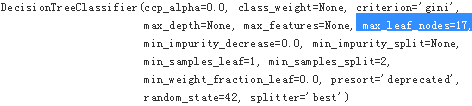
d. Train it on the full training set using these hyperparameters, and measure your model’s performance on the test set. You should get roughly 85% to 87% accuracy.
By default, GridSearchCV trains the best model found on the whole training set (you can change this by setting refit=False), so we don't need to do it again. We can simply evaluate the model's accuracy:
from sklearn.metrics import accuracy_score

y_pred = grid_search_cv.predict(X_test)
accuracy_score(y_test, y_pred) ![]()
8. Grow a forest.
a. Continuing the previous exercise, generate 1,000 subsets of the training set, each containing 100 instances selected randomly. Hint: you can use Scikit- Learn’s ShuffleSplit class for this.
from sklearn.model_selection import ShuffleSplit
#n_samples=10000
#test_size=0.2   len(X_test)=2000   len(X_train)=8000
n_trees = 1000
n_instances = 100

mini_sets = []
                                    #len(variation set OR test_size)=8000-100=7900 then sub_training set size=100
rs = ShuffleSplit(n_splits=n_trees, test_size=len(X_train)- n_instances, random_state=42)
for mini_train_index, mini_test_index in rs.split(X_train):
    X_mini_train = X_train[mini_train_index] #length=100
    y_mini_train = y_train[mini_train_index]
    mini_sets.append( (X_mini_train,y_mini_train) )
b. Train one Decision Tree on each subset, using the best hyperparameter values found above. Evaluate these 1,000 Decision Trees on the test set. Since they were trained on smaller sets, these Decision Trees will likely perform worse than the first Decision Tree, achieving only about 80% accuracy.
from sklearn.base import clone

forest = [ clone(grid_search_cv.best_estimator_) for _ in range(n_trees) ] #length==1000
forest[:3]
accuracy_scores = []

for tree, (X_mini_train, y_mini_train) in zip(forest, mini_sets):
    tree.fit(X_mini_train, y_mini_train)

    y_pred = tree.predict(X_test)
    accuracy_scores.append( accuracy_score(y_test, y_pred) )

np.mean( accuracy_scores )![]()
Since they were trained on smaller sets(size=100), these Decision Trees will likely perform worse than the first Decision Tree, achieving only about 80% accuracy.
c. Now comes the magic. For each test set instance, generate the predictions of the 1,000 Decision Trees, and keep only the most frequent prediction (you can use SciPy’s mode() function for this). This gives you majority-vote predictions over the test set.
# n_trees = 1000
Y_pred = np.empty( [n_trees, len(X_test)], dtype=np.uint8 ) #(1000, 2000)

for tree_index, tree in enumerate(forest):
    Y_pred[tree_index] = tree.predict(X_test)

from scipy.stats import mode
y_pred_majority_votes, n_votes = mode(Y_pred, axis=0)
y_pred_majority_votes, n_votes![]()
d. Evaluate these predictions on the test set: you should obtain a slightly higher accuracy than your first model (about 0.5 to 1.5% higher). Congratulations, you have trained a Random Forest classifier!
accuracy_score( y_test, y_pred_majority_votes.reshape([-1]) )![]()
########################################extra materials
Tree Pruning树的剪枝 (from "An Introduction to Statistical Learning")
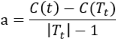
The process described above(decision tree) may produce good predictions on the training set, but is likely to overfit the data, leading to poor test set performance. This is because the resulting tree might be too complex. A smaller tree with fewer splits (that is, fewer regions ![]() ) might lead to lower variance and better interpretation at the cost of a little bias. One possible alternative to the process described above is to build the tree only so long as the decrease in the RSS due to each split exceeds some (high) threshold. This strategy will result in smaller trees, but is too short-sighted since a seemingly worthless split early(早期RSS并没有大幅减小) on in the tree might be followed by a very good split—that is, a split that leads to a large reduction in RSS later on (RSS大幅减小).
) might lead to lower variance and better interpretation at the cost of a little bias. One possible alternative to the process described above is to build the tree only so long as the decrease in the RSS due to each split exceeds some (high) threshold. This strategy will result in smaller trees, but is too short-sighted since a seemingly worthless split early(早期RSS并没有大幅减小) on in the tree might be followed by a very good split—that is, a split that leads to a large reduction in RSS later on (RSS大幅减小).
Therefore, a better strategy is to grow a very large tree ![]() ( and also use a stopping criterion based on the number
( and also use a stopping criterion based on the number
of data points associated with the leaf nodes), and then prune it back in order to obtain a subtree. How do we determine the best prune way to prune the tree? Intuitively, our goal is to select a subtree that subtree leads to the lowest test error rate. Given a subtree, we can estimate its test error using cross-validation or the validation set approach. However, estimating the cross-validation error for every possible subtree would be too cumbersome, since there is an extremely large number of possible subtrees. Instead, we need a way to select a small set of subtrees for consideration.
(more times of spliting a dataset, larger size to the tree, more number of leaf nodes(and each leaf may just contain fewer data points or samples) and the model become more complexity, but minimizes residual errors )
############################
The pruning is based on a criterion that balances residual error against a measure of model complexity. If we denote the starting tree for pruning by ![]() , then we define
, then we define ![]() to be a subtree of
to be a subtree of ![]() if it can be obtained by pruning nodes from
if it can be obtained by pruning nodes from ![]() (in other words, by collapsing折叠 internal nodes by combining the corresponding regions即通过合并对应区域来收缩内部结点). Suppose the leaf nodes are indexed by τ = 1, . . . , |T|, with leaf node τ representing a region
(in other words, by collapsing折叠 internal nodes by combining the corresponding regions即通过合并对应区域来收缩内部结点). Suppose the leaf nodes are indexed by τ = 1, . . . , |T|, with leaf node τ representing a region ![]() of input space having
of input space having ![]() data points(samples), and |T| denoting the total number of leaf nodes. The optimal prediction for region
data points(samples), and |T| denoting the total number of leaf nodes. The optimal prediction for region ![]() is then given by 那么区域
is then given by 那么区域![]() 给出的最优的预测为
给出的最优的预测为 
and the corresponding contribution to the residual sum-of-squares is then ![]()
The pruning criterion is then given by 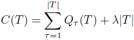 (minimizing)
The regularization parameter λ determines the trade-off between the overall residual sum-of-squares error and the complexity of the model as measured by the number |T| of leaf nodes, and its value is chosen by cross-validation.
########################################################
Understanding:
When λ = 0, then the subtree T will simply equal 原树 ![]() (the model is optimal), because then (8.4) just measures the training error(
(the model is optimal), because then (8.4) just measures the training error(![]() ). When λ increases a little bit, |T| is large, and the complexity of the model is increasing (the variance is higher but low-bias; When λ increases a lot, |T| is small, and the complexity of the model is decreasing (the variance is lower but high-bias; When λ -->∞, the root node is the only node in the optimal tree.
). When λ increases a little bit, |T| is large, and the complexity of the model is increasing (the variance is higher but low-bias; When λ increases a lot, |T| is small, and the complexity of the model is decreasing (the variance is lower but high-bias; When λ -->∞, the root node is the only node in the optimal tree.
为了得到所有的可能生成的最优化树{![]() ,T1,T2,…Tn},我们须从底向上(从最近叶子节点的internal node到root根节点),每次进行一次剪枝,通过得到的树认为是最优化树反推λ; 具体的,从整体树
,T1,T2,…Tn},我们须从底向上(从最近叶子节点的internal node到root根节点),每次进行一次剪枝,通过得到的树认为是最优化树反推λ; 具体的,从整体树![]() 开始剪枝,对于
开始剪枝,对于![]() 的任意internal node t(内部结点t),结点下有若干子节点,把internal node t 下的子树的若干leaf node called Tt (叶节点称为Tt)。
的任意internal node t(内部结点t),结点下有若干子节点,把internal node t 下的子树的若干leaf node called Tt (叶节点称为Tt)。
剪枝前的损失函数 ==> ![]()
剪枝后(即internal node t下的子树(即若干leaf node )减去后,internal node t 变为leaf node叶节点)的损失函数
![]()
注意这里的损失函数![]() 都是某个叶结点的损失函数,但为什么可以只求叶节点的损失函数,因为在 ID3,C4.5中得出了C(T)作为模型的预测误差的值,通过累加每一个叶结点(即T个叶结点)的预测误差而得出C(T)。因此单独求某个叶结点并没有什么问题。
都是某个叶结点的损失函数,但为什么可以只求叶节点的损失函数,因为在 ID3,C4.5中得出了C(T)作为模型的预测误差的值,通过累加每一个叶结点(即T个叶结点)的预测误差而得出C(T)。因此单独求某个叶结点并没有什么问题。
现在就是求解a,a如何求解?
- 当a=0或充分小时(OR λ=0 or enough small),不等式 (剪枝前的损失函数)
 (剪枝后的损失函数), 因为叶结点越多预测误差应该越小(unpruned tree: higher variance but low-bias(
 <
< ))。
))。 - 当a (OR λ) 不断增大时(想一下,剪掉一个叶子节点,|T|减小,a变大,变大成为),在某个a点有个平衡
- 当a再增大时,不等式反向。
- 因此只要
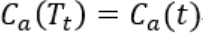
Tt与t有相同的损失函数(![]() ),而t结点少,因此t比Tt更可取,对Tt进行剪枝。
),而t结点少,因此t比Tt更可取,对Tt进行剪枝。
接下来对![]() 这棵整体树中的每一个结点t,计算
这棵整体树中的每一个结点t,计算 
OR ![]() when you prune all leaf nodes under the t, then
when you prune all leaf nodes under the t, then ![]() =1 (internal node t 变为leaf node叶节点) https://en.wikipedia.org/wiki/Decision_tree_pruning
=1 (internal node t 变为leaf node叶节点) https://en.wikipedia.org/wiki/Decision_tree_pruning
这个g(t)表示剪枝后的整体损失函数减少程度,实际上可以看为是否剪枝的阈值,对于某个结点当他的参数a=g(t)时,剪和不剪总体损失函数时一样的。如果a增大则不剪的整体损失函数就大于剪去的。即a>g(t)该剪,剪后会使整体损失函数减小,而a<g(t)则不剪,剪后会使整体损失函数增大。
这样a缓慢增大,随着a的增大,在一个区间内可确定一棵最优的剪枝树
而我们求每棵树,并认为他是最优剪枝树。
g(t)则代表每一棵树的a的最优区间内的最小值
即在T0中剪去g(t)最小的Tt,得到的子树为T1,同时将最小的g(t)设为a1,那么T1为区间[a1,a2)的最优子树。
如此这样下去,将所有可能的树的情况剪枝直到根节点,在这个过程中则 会不断增加a,产生新的区间,最后a的所有可能的g(t)取值全部确定。
2.通过交叉验证选取最优子树
具体的利用独立的验证数据集,测试子树序列T0,T1,…Tn中各棵子树的平方误差![]() 或基尼指数。平方误差或基尼指数最小的决策树被认为是最优决策树,因为我们每确定一棵子树就会确定其参数a值
或基尼指数。平方误差或基尼指数最小的决策树被认为是最优决策树,因为我们每确定一棵子树就会确定其参数a值![]() ,所以最优子树Tk确定,对应ak也确定,即得到最优决策数Ta。
,所以最优子树Tk确定,对应ak也确定,即得到最优决策数Ta。
########################################################
############################
Cost complexity pruning代价复杂性剪枝—also known as weakest link pruning最弱联系剪枝—gives us a way to do just this. Rather than considering every possible subtree, we consider a sequence of trees indexed by a nonnegative tuning parameter α. For each value of α there corresponds a subtree ![]() such that
such that ![]() is as small as possible. Here |T | indicates the number of terminal nodes(or leaves) of the tree T ,
is as small as possible. Here |T | indicates the number of terminal nodes(or leaves) of the tree T , ![]() is the rectangle (i.e. the subset of predictor space) corresponding to the mth terminal node, and
is the rectangle (i.e. the subset of predictor space) corresponding to the mth terminal node, and ![]() is the predicted response associated with
is the predicted response associated with ![]() —that is, the mean of the training observations in
—that is, the mean of the training observations in ![]() . The tuning parameter α controls a trade-off between the subtree's complexity and its fit to the training data. When α = 0, then the subtree T will simply equal 原树
. The tuning parameter α controls a trade-off between the subtree's complexity and its fit to the training data. When α = 0, then the subtree T will simply equal 原树 ![]() , because then (8.4) just measures the training error. However, as α increases, there is a price to pay for having a tree with many terminal nodes, and so the quantity (8.4 ) will tend to be minimized for a smaller subtree. Equation 8.4 is reminiscent使人联想…的 of the lasso (6.7
, because then (8.4) just measures the training error. However, as α increases, there is a price to pay for having a tree with many terminal nodes, and so the quantity (8.4 ) will tend to be minimized for a smaller subtree. Equation 8.4 is reminiscent使人联想…的 of the lasso (6.7  ) from Chapter 6, in which a similar formulation was used in order to control the complexity of a linear model.
It turns out that as we increase α from zero in (8.4 ), branches get pruned from the tree in a nested and predictable fashion方式, so obtaining the whole sequence of subtrees as a function of α is easy. We can select a value of α using a validation set or using cross-validation. We then return to the full data set and obtain the subtree corresponding to α. This process is summarized in Algorithm 8.1.

Algorithm 8.1 Building a Regression Tree
- Use recursive binary splitting to grow a large tree on the training data, stopping only when each terminal node has fewer than some minimum number of observations.
- Apply cost complexity pruning
minimize to the large tree in order to obtain a sequence of best subtrees一系列最优子树, as a function of α-子树是α 的函数。pick α to minimize the average error - Use K-fold cross-validation to choose α. That is, divide the training observations(if size =132) into K folds( If K=6). For each k = 1, . . .,K:
(a) Repeat Steps 1 and 2 on all but the kth fold(validation set) of the training data. (对训练集所有不属于第k 折(validation set)的数据重复步骤1 (grow a tree)和2(pruning) ,得到与 α --对应的子树
Suggestion: if you cut the internal node which is the nearest to the leaf nodes, you don't repreat steps1 and 2
上这操作结束后,每个α 会有相应的K 个均方预测误差,对这K个均方预测误差求平均值(是α 的函数),选出使平均误差最小的α。 - (b) Evaluate the mean squared prediction error on the data in the left-out kth fold, as a function of α.
Average the results(MSE) for each value of α, and pick α to minimize the average error - Return the subtree from Step 2 that corresponds to the chosen value of α.

FIGURE 8.4. Regression tree analysis for the Hitters data. The unpruned tree that results from top-down greedy splitting on the training data is shown.
Figures 8.4 and 8.5 display the results of fitting and pruning a regression tree on the Hitters data, using nine of the features(Years, RBI, Hits, Putout, Years for leaf nodes, Walks, Runs, RBI, Years for leaf node). First, we randomly
divided the data set in half, yielding 132 observations in the training set and 131 observations in the test set. We then built a large regression tree on the training data and varied α in (8.4 ) in order to create subtrees with different numbers of terminal nodes. Finally, we performed six-fold crossvalidation in order to estimate the cross-validated MSE of the trees as a function of α. (We chose to perform six-fold cross-validation because
132 is an exact multiple of six.) The unpruned regression tree is shown in Figure 8.4.
FIGURE 8.5. Regression tree analysis for the Hitters data. The training(bottom), cross-validation(green curve, top), and test MSE(middle) are shown as a function of the number of terminal nodes in the pruned tree. Standard error bands are displayed. The minimum cross-validation error occurs at a tree size of three.
The green curve in Figure 8.5 shows the CV(cross-validation) error as表示为 a function of the number of leaves, while the orange curve indicates the test error. Also shown are standard error bars around the estimated errors. For reference, the training error curve is shown in black. The CV error is a reasonable approximation![]() of the test error: the CV error takes on its minimum for a three-node tree, while the test error also dips down at the three-node tree (though it takes on its lowest value at the ten-node tree). The pruned tree containing three terminal nodes is shown in Figure 8.1.
of the test error: the CV error takes on its minimum for a three-node tree, while the test error also dips down at the three-node tree (though it takes on its lowest value at the ten-node tree). The pruned tree containing three terminal nodes is shown in Figure 8.1.
8.1.2 Classification Trees
A classification tree is very similar to a regression tree, except that it is classification used to predict a qualitative定性 response rather than a quantitative定量one. Re-call that for a regression tree, the predicted response for an observation is given by the mean response(RSS: , ![]() is the mean(or average) response for the training observations within the
is the mean(or average) response for the training observations within the ![]() box/region) of the training observations that belong to the same terminal node(called leaf node/region). In contrast, for a classification tree, we predict that each observation belongs to the most commonly occurring class of training observations in the region to which it belongs. In interpreting the results of a classification tree, we are often interested not only in the class prediction corresponding to a particular terminal node region, but also in the class proportions各个类所占的比例 among the training observations that fall into that region.
box/region) of the training observations that belong to the same terminal node(called leaf node/region). In contrast, for a classification tree, we predict that each observation belongs to the most commonly occurring class of training observations in the region to which it belongs. In interpreting the results of a classification tree, we are often interested not only in the class prediction corresponding to a particular terminal node region, but also in the class proportions各个类所占的比例 among the training observations that fall into that region.
The task of growing a classification tree is quite similar to the task of growing a regression tree. Just as in the regression setting, we use recursive binary splitting递归二叉分裂 to grow a classification tree. However, in the classification setting, RSS cannot be used as a criterion for making the binary splits. A natural alternative to RSS is the classification error rate分类错误率. Since we plan classification to assign an observation in a given region to the most commonly occurring class of training observations in that region, the classification error rate is simply the fraction比例 of the training observations in that region that do not belong to the most common class: ![]()
Here ![]() represents the proportion of training observations in the mth region that are from the kth class. However, it turns out that classification error is not sufficiently sensitive for tree-growing, and in practice two other measures are preferable.
represents the proportion of training observations in the mth region that are from the kth class. However, it turns out that classification error is not sufficiently sensitive for tree-growing, and in practice two other measures are preferable.
https://blog.csdn.net/Linli522362242/article/details/104542381 see above content
The Gini index is defined by 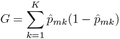
a measure of total variance总方差![]() across the K classes. It is not hard to see that the Gini index takes on a small value if all of the ˆpmk’s are close to zero or one. For this reason the Gini index is referred to as a measure of
across the K classes. It is not hard to see that the Gini index takes on a small value if all of the ˆpmk’s are close to zero or one. For this reason the Gini index is referred to as a measure of
node purity—a small value indicates that a node contains predominantly observations from a single class.
An alternative to the Gini index is cross-entropy互熵, given by 
Since ![]() , it follows that
, it follows that ![]() . One can show that the cross-entropy will take on a value near zero if the
. One can show that the cross-entropy will take on a value near zero if the ![]() s are all near zero or near one. Therefore, like the Gini index, the cross-entropy will take on a small value if the mth node is pure. In fact, it turns out that the Gini index and the cross-entropy are quite similar numerically.
s are all near zero or near one. Therefore, like the Gini index, the cross-entropy will take on a small value if the mth node is pure. In fact, it turns out that the Gini index and the cross-entropy are quite similar numerically.
When building a classification tree, either the Gini index or the cross entropy are typically used to evaluate the quality品质 of a particular split, since these two approaches are more sensitive to node purity than is the classification error rate. Any of these three approaches might be used when pruning the tree, but the classification error rate![]() is preferable if prediction accuracy of the final pruned tree is the goal.
is preferable if prediction accuracy of the final pruned tree is the goal.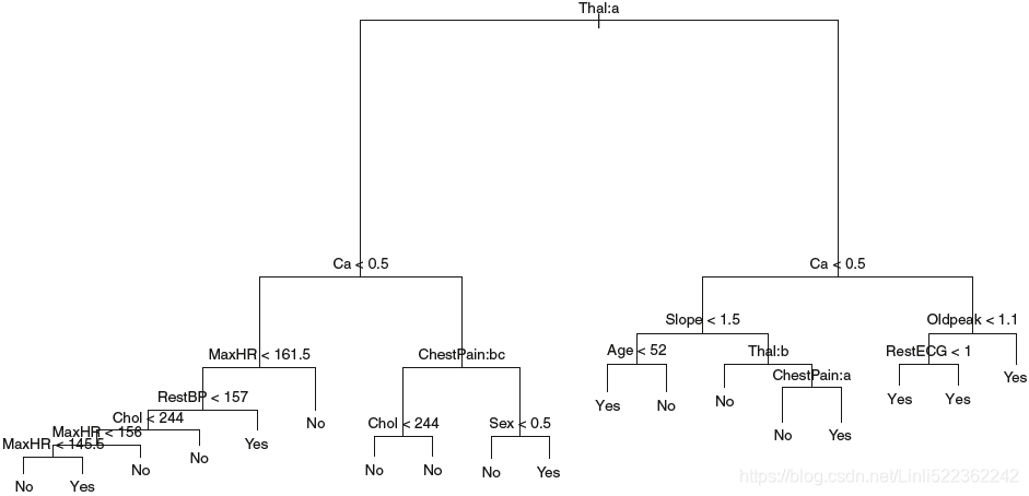

FIGURE 8.6. Heart data. Top: The unpruned tree. Bottom Left: Cross -validation error, training, and test error, for different sizes of the pruned tree. Bottom Right: The pruned tree corresponding to the minimal cross-validation error.
Figure 8.6 shows an example on the Heart data set. These data contain a binary outcome HD(Heart Disease) for 303 patients who presented with chest pain. An outcome value of Yes indicates the presence of heart disease based on
an angiographic test经血管造影诊断, while No means no heart disease. There are 13 predictors including Age, Sex, Chol (a cholesterol measurement(胆固醇指标)), and other heart and lung function measurements. Cross-validation results in a tree with six terminal nodes.
In our discussion thus far, we have assumed that the predictor variables take on continuous values(for quantative定量 #regression tree). However, decision trees can be constructed even in the presence of qualitative定性 predictor variables(#classification). For instance, in the Heart data, some of the predictors, such as Sex, Thal (Thalium stress test压力测试), and ChestPain, are qualitative. Therefore, a split on one of these variables amounts to assigning some of the qualitative values to one branch and assigning the remaining to the other branch. In Figure 8.6, some of the internal
nodes correspond to splitting qualitative variables. For instance, the top internal node corresponds to splitting Thal. The text Thal:a indicates that the left-hand branch coming out of that node consists of observations with the first value of the Thal variable (normal), and the right-hand node consists of the remaining observations (fixed or reversible defects). The text ChestPain:bc two splits down the tree on the left indicates that the left-hand branch coming out of that node consists of observations with the second and third values of the ChestPain variable, where the possible values are
typical angina典型心绞痛, atypical angina非典型心绞痛, non-anginal pain非心疼痛, and asymptomatic无临床症状.
Figure 8.6 has a surprising characteristic: some of the splits yield two terminal nodes that have the same predicted value. For instance, consider the split RestECG<1  near the bottom right of the unpruned tree. Regardless
of不论 the value of RestECG, a response value of Yes is predicted for those observations. Why, then, is the split performed at all? The split is performed because it leads to increased node purity. That is, all 9 of the observations corresponding to the right-hand leaf have a response value of Yes, whereas 7/11 of those corresponding to the left-hand leaf have a response value of Yes. Why is node purity important? Suppose that we have a test observation that belongs to the region given by that right-hand leaf. Then we can be pretty certain that its response value is Yes. In contrast, if a test
observation belongs to the region given by the left-hand leaf, then its response value is probably Yes, but we are much less certain. Even though the split RestECG<1 does not reduce the classification error, it improves the Gini index and the cross-entropy, which are more sensitive to node purity.
8.1.3 Trees Versus Linear Models
Regression and classification trees have a very different flavor from the more classical approaches for regression and classification. In particular, linear regression assumes a model of the form 
whereas regression trees assume a model of the form 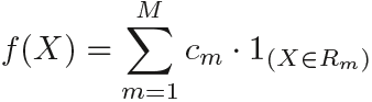
Note: ![]() is the actual response
is the actual response
where R1, . . .,RM represent a partition of feature space, as in Figure 8.3.
####################### for understanding ![]()

#######################
Which model is better? It depends on the problem at hand. If the relationship between the features and the response is well approximated by a linear model as in (8.8 ), then an approach such as linear regression
will likely work well, and will outperform a method such as a regression tree that does not exploit this linear structure. If instead there is a highly non-linear and complex relationship between the features and the response as indicated by model (8.9 ), then decision trees may outperform classical approaches. An illustrative example is displayed in Figure 8.7. The relative performances of tree-based and classical approaches can be assessed by estimating the test error, using either cross-validation or the validation set approach.

FIGURE 8.7. Top Row: A two-dimensional classification example in which the true decision boundary is linear, and is indicated by the shaded regions. A classical approach that assumes a linear boundary (left) will outperform a decision
tree that performs splits parallel to the axes (right). Bottom Row: Here the true decision boundary is non-linear. Here a linear model is unable to capture the true decision boundary (left), whereas a decision tree is successful (right).
8.1.4 Advantages and Disadvantages of Trees
Decision trees for regression and classification have a number of advantages over the more classical approaches:
- Trees are very easy to explain to people. In fact, they are even easier to explain than linear regression!
- Some people believe that decision trees more closely mirror human decision-making than do the regression and classification approaches.
- Trees can be displayed graphically, and are easily interpreted even by a non-expert (especially if they are small).
- Trees can easily handle qualitative定性 predictors without the need to create dummy variables.
- Unfortunately, trees generally do not have the same level of predictive accuracy as some of the other regression and classification approaches.
However, by aggregating many decision trees, using methods like bagging, random forests, and boosting, the predictive performance of trees can be substantially improved. We introduce these concepts in the next section.
