CAM(Class Activation Mapping)

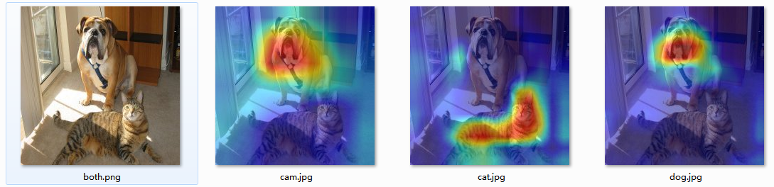
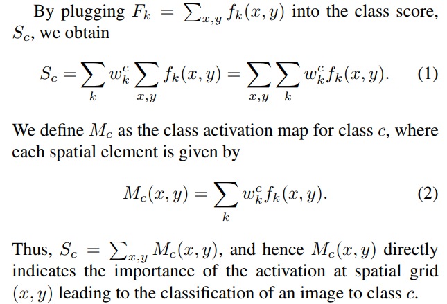
CAM出自于论文 Learning Deep Features for Discriminative Localization（CVPR2016）

以热力图的形式展示，模型通过哪些像素点得知图片属于某个类别。

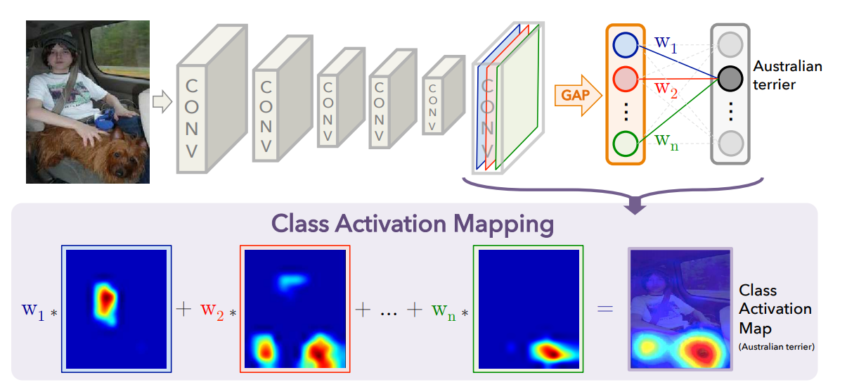
论文中原句：before the final output layer (softmax in the case of categorization), we perform global average pooling on the convolutional feature maps and use those as features for a fully-connected layer that produces the desired output (categorical or otherwise)

关于GAP(Global Average Pooling)，详见另一篇博客：https://blog.csdn.net/qq_21097885/article/details/90018322

​​

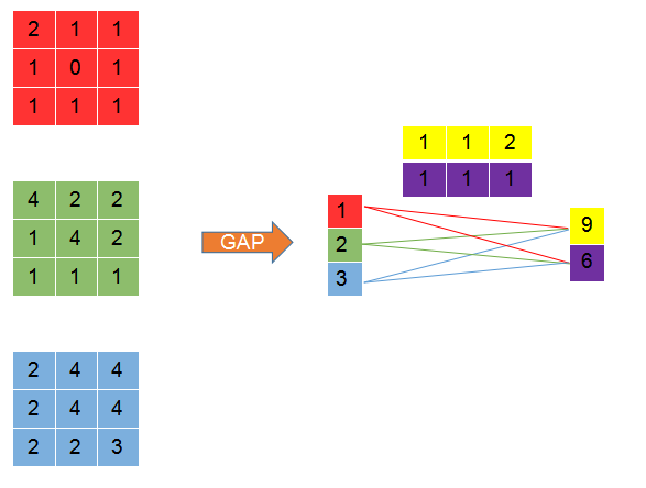
举个例子，卷积最后得到的特征图为 $3 \times 3 \times 3$。
第一个特征图经过GAP(Global Average Pooling)，得到 $(2+1+1+1+0+1+1+1+1) / 9 = 1$。同理，第二个特征图经过GAP得到2，第三个特征图经过GAP得到3。
经过全连接层，得到二分类的结果为（9, 6）.
Softmax之后，得到（0.6, 0.4）.

仔细分析一下，二分类结果中9是如何得到的。

$1 \times [ (2+1+1+1+0+1+1+1+1) / 9 ] + 1 \times [ (4+2+2+1+4+2+1+1+1) / 9 ] + 2 \times [ (2+4+4+2+4+4+2+2+3) / 9 ] = 9$

也就是 $W_{11} * \frac{\sum F_{1}}{9}+W_{12} * \frac{\sum F_{2}}{9}+W_{13} * \frac{\sum F_{3}}{9}$

写为 $\frac{\sum (W_{11}*F_{1}+W_{12}*F_{2}+W_{13}*F_{3})}{9}$

即， $\frac{(10 + 11 + 11+6+12+11+6+6+8)}{9} = 9$

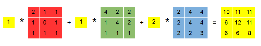
各个像素点对最后分类为第一类的贡献值为 $\left\{ \begin{matrix} 10 & 11 & 11 \\ 6 & 12 & 11 \\ 6 & 6 & 8 \end{matrix} \right\}$
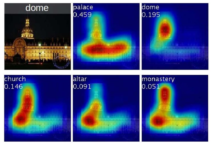
这样，就可以得到热力图了。最后，将该热力图暴力展开成所需要的大小即可。叠加到原图中，就可以观察模型得到的分类结果关注于图片中哪个区域了。

对应论文中解释

下图中图片的标签是“圆顶”。五张类激活映射分别是前五名预测的类别和得分。可以看到，预测为“宫殿”时，模型关注于整个区域。预测为“圆顶”时，模型只关注于宫殿顶部。

源码：https://github.com/metalbubble/CAM

缺陷：必须改变网络结构，例如把全连接层改成全局平均池化层。

后出现改进的技术Grad-CAM，详见这篇论文 Grad-CAM: Visual Explanations from Deep Networks via Gradient-based Localization ( ICCV2017)。