import modules 导入模块
import statsmodels as sm  # used in machine learning 用于机器学习
import seaborn as sns # a visualization library 一个可视化库
import numpy as np # a module for performing mathematical operations on lists of data 一个对表格进行数据运算的模块
CASE: looking for Bayes’ kidnapper
案例:查找绑架Bayes的绑架者
1. fill out a Missing Puppy Report with details of the case 填写丢失报告
bayes_age = 4.0
favorite_toy = "Mr. Squeaky"
owner = 'DataCamp'
# single or double quotes would be OK
fur_color = "blonde"
birthday = "2017-07-14"
case_id = 'DATACAMP!123-456?'
# Variable names cannot begin with a number
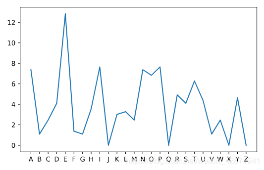
2. ransom note 勒索信
analyze the frequency with which each letter occurs in the note
分析勒索信中每一个字母出现的频率
import pandas as pd
r = pd.read_csv('ransom.csv')
print(r)

    letter_index letter  frequency  # percent
0              1      A       7.38
1              2      B       1.09
2              3      C       2.46
3              4      D       4.10
4              5      E      12.84
               ...
21            22      V       1.09
22            23      W       2.46
23            24      X       0.00
24            25      Y       4.64
25            26      Z       0.00
plt.plot(x_values, y_values)
plt.show()
3. Snooping for suspects 发现嫌疑人
A witness noticed: a green truck leaving the scene of the crime whose license plate began with ‘FRQ’
一个目击者声称发现一辆绿色卡车驶离犯罪现场,车牌开头字母为 ‘FRQ’
plate = 'FRQ****'
lookup_plate(plate, color = 'Green')

<script.py> output:

      Fred Frequentist
      Ronald Aylmer Fisher
      Gertrude Cox
      Kirstine Smith
4. credit card records 犯罪嫌疑人的信用卡记录
We’ve obtained credit card records for all four suspects. Perhaps some of them made suspicious purchases before the kidnapping?
我们已经获得了四位犯罪嫌疑人的信用卡记录。或许他们其中有人在绑架前存在一些可以购买。
import pandas as pd
credit_records = pd.read_csv('credit_records.csv')
print(credit_records.head()) # 显示credit_records的前5行

<script.py> output:
                suspect         location              date         item  price
    0    Kirstine Smith   Groceries R Us   January 6, 2018     broccoli   1.25
    1      Gertrude Cox  Petroleum Plaza   January 6, 2018  fizzy drink   1.90
    2  Fred Frequentist   Groceries R Us   January 6, 2018     broccoli   1.25
    3      Gertrude Cox   Groceries R Us  January 12, 2018     broccoli   1.25
    4    Kirstine Smith    Clothing Club   January 9, 2018        shirt  14.25
Use the .info() method to inspect the DataFrame credit_records
使用.info()检查credit_records
print(credit_records.info())

<script.py> output:
    <class 'pandas.core.frame.DataFrame'>
    RangeIndex: 104 entries, 0 to 103
    Data columns (total 5 columns):
    suspect     104 non-null object
    location    104 non-null object
    date        104 non-null object
    item        104 non-null object
    price       104 non-null float64
    dtypes: float64(1), object(4)
    memory usage: 4.1+ KB
    None
Let’s examine the items that they’ve purchased.
让我们检查一下他们购买的物品。
items = credit_records["item"] # Method 1
print(items)

items = credit_records.item # Method 2
print(items)

<script.py> output:
    0          broccoli
    1       fizzy drink
    2          broccoli
    3          broccoli
    4             shirt
               ...
    99            shirt
    100           pants
    101           dress
    102          burger
    103       cucumbers
    Name: item, Length: 104, dtype: object
5. Selecting missing puppies 选择丢失的幼犬
Examining Missing Puppy Reports
查看丢失幼犬报告
print(mpr.info())
name = mpr["Dog Name"] # 列名包含空格,只能用方法一
is_missing = mpr["Missing?"]
print(name)
print(is_missing)

<script.py> output:
    <class 'pandas.core.frame.DataFrame'>
    RangeIndex: 4 entries, 0 to 3
    Data columns (total 4 columns):
    Dog Name      4 non-null object
    Owner Name    4 non-null object
    Dog Breed     4 non-null object
    Missing?      4 non-null object
    dtypes: object(4)
    memory usage: 208.0+ bytes
    None

0      Bayes
1    Sigmoid
2     Sparky
3    Theorem
Name: Dog Name, dtype: object

0    Still Missing
1    Still Missing
2            Found
3            Found
Name: Missing?, dtype: object
Let’s select a few different rows to learn more about the other missing dogs.
让我们选择一些不同的行以便于了解更多关于其他丢失幼犬的信息。
greater_than_2 = mpr[mpr.Age > 2]
print(greater_than_2)

still_missing = mpr[mpr.Status == 'Still Missing']
print(still_missing)

not_poodle = mpr[mpr['Dog Breed'] != 'Poodle']
print(not_poodle)

<script.py> output:
      Dog Name             Owner Name       Dog Breed Status  Age
    2   Sparky             Dr. Apache   Border Collie  Found    3
    3  Theorem  Joseph-Louis Lagrange  French Bulldog  Found    4
    5    Benny   Hillary Green-Lerman          Poodle  Found    3

      Dog Name    Owner Name         Dog Breed         Status  Age
    0    Bayes      DataCamp  Golden Retriever  Still Missing    1
    1  Sigmoid                       Dachshund  Still Missing    2
    4      Ned  Tim Oliphant          Shih Tzu  Still Missing    2

      Dog Name             Owner Name         Dog Breed         Status  Age
    0    Bayes               DataCamp  Golden Retriever  Still Missing    1
    1  Sigmoid                                Dachshund  Still Missing    2
    2   Sparky             Dr. Apache     Border Collie          Found    3
    3  Theorem  Joseph-Louis Lagrange    French Bulldog          Found    4
    4      Ned           Tim Oliphant          Shih Tzu  Still Missing    2
6. Narrowing the list of suspects 缩小犯罪嫌疑人名单
We’d like to know if any of them recently purchased dog treats to use in the kidnapping. If they did, they would have visited ‘Pet Paradise’.
我们想要了解在绑架前是否有人购买了狗粮,如果有人购买,他们会去’Pet Paradise’。
purchase = credit_records[credit_records.location == 'Pet Paradise']
print(purchase)

<script.py> output:
                 suspect      location              date          item  price
    8   Fred Frequentist  Pet Paradise  January 14, 2018    dog treats   8.75
    9   Fred Frequentist  Pet Paradise  January 14, 2018    dog collar  12.25
    28      Gertrude Cox  Pet Paradise  January 13, 2018  dog chew toy   5.95
    29      Gertrude Cox  Pet Paradise  January 13, 2018    dog treats   8.75
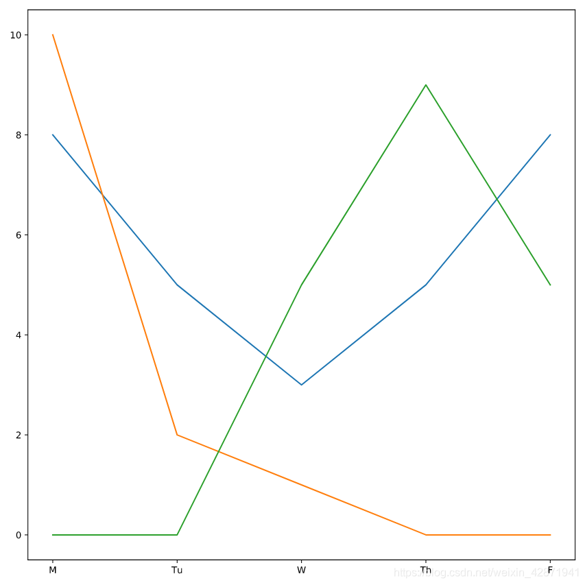
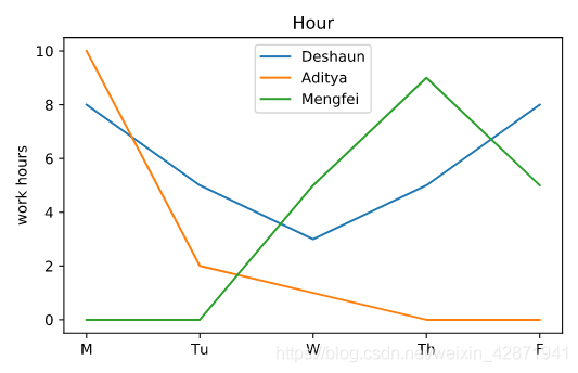
7. Working hard or hardly working? 警官是否努力工作?
Tracking the amount of time he spent working on this case.
Deshaun警官查看他在这个案件上花费的工作时间。
from matplotlib import pyplot as plt
plt.plot(deshaun.day_of_week, deshaun.hours_worked)
plt.show()

We’ll plot all three lines together to see who was working hard each day.
我们将查看一下三位警官每天在该案件上花费的时长。

plt.plot(deshaun.day_of_week, deshaun.hours_worked)
plt.plot(aditya.day_of_week, aditya.hours_worked)
plt.plot(mengfei.day_of_week, mengfei.hours_worked)
plt.show()
Adding a legend to distinguish the three lines.
添加一个图例来区别三条线。
plt.plot(deshaun.day_of_week, deshaun.hours_worked, label='Deshaun')
plt.plot(aditya.day_of_week, aditya.hours_worked, label='Aditya')
plt.plot(mengfei.day_of_week, mengfei.hours_worked, label='Mengfei')
plt.legend() # 添加图例
plt.show()
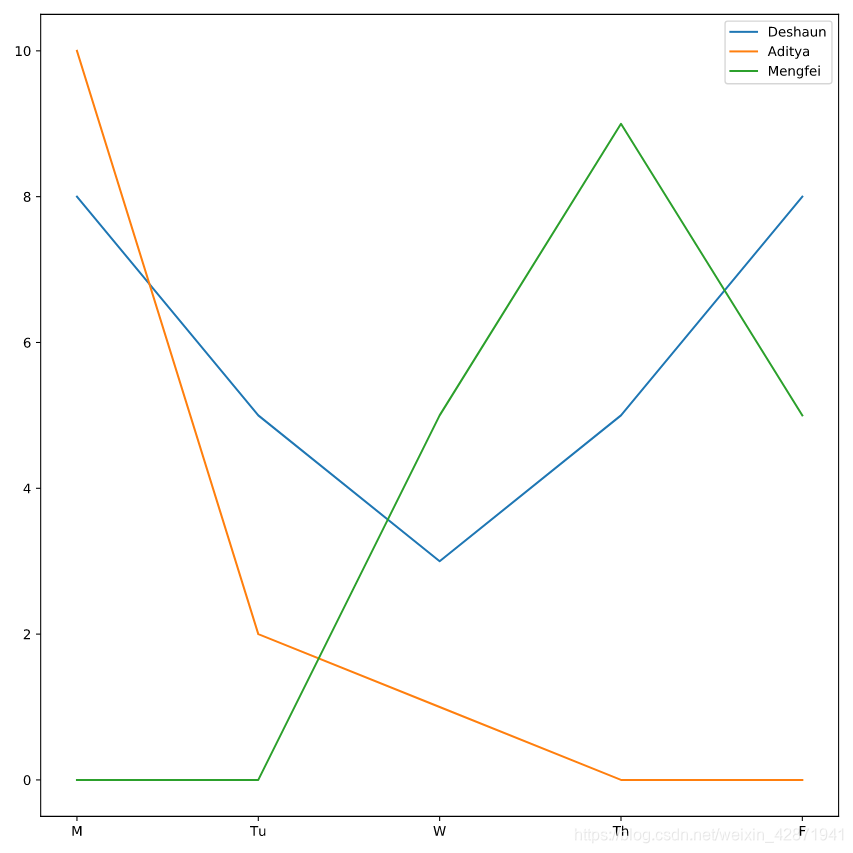
If we give a chart with no labels to Officer Deshaun’s supervisor, she won’t know what the lines represent. We need to add labels to Officer Deshaun’s plot of hours worked.
如果我们没有添加标签,Deshaun警官的上司就无法明白图表的含义。我们需要为这个图表添加标签。
plt.plot(deshaun.day_of_week, deshaun.hours_worked, label='Deshaun')
plt.plot(aditya.day_of_week, aditya.hours_worked, label='Aditya')
plt.plot(mengfei.day_of_week, mengfei.hours_worked, label='Mengfei')
plt.title('Hour') # 添加标题
plt.ylabel('work hours') # 添加Y轴标签
plt.legend()
plt.show()
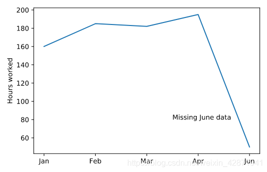
Officer Deshaun is examining the number of hours that he worked over the past six months. The number for June is low because he only had data for the first week. Help Deshaun add an annotation to the graph to explain this.
Deshaun警官正在检查他最近6个月的工作时间,其中6月的数值比较低的原因师他只有6月第1周的数据。我们需要添加一个注释去解释数据异常的原因。
plt.plot(six_months.month, six_months.hours_worked)
plt.text(2.5, 80, "Missing June data") # 添加注释
plt.show()
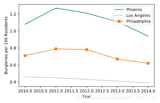
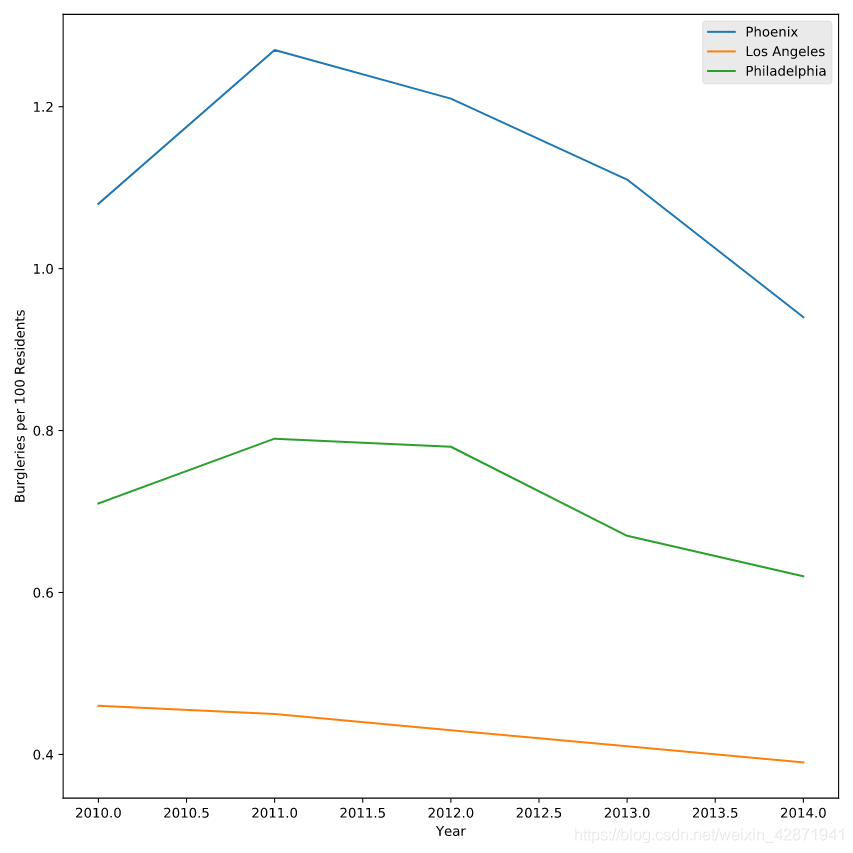
8. Tracking crime statistics 追踪犯罪统计数据
Laura has plotted Burglary rates in three U.S. cities using data from the Uniform Crime Reporting Statistics.
Laura警官利用统一犯罪报告统计数据绘制了美国三个城市的入室盗窃率。
plt.plot(data["Year"], data["Phoenix Police Dept"], label="Phoenix", color = 'DarkCyan')
plt.plot(data["Year"], data["Los Angeles Police Dept"], label="Los Angeles", linestyle = ':')
# 线型:虚线(':','--'),实线('')
plt.plot(data["Year"], data["Philadelphia Police Dept"], label="Philadelphia", marker = 's')
# 标记:圆形('o'),菱形('d'),方形('s')
plt.legend()
plt.show()
Changing the plotting style is a fast way to change the entire look of your plot without having to update individual colors or line styles.
更改绘图样式是一种快速的方法,可以更改整个绘图的外观,而不必更新单独的颜色或线条样式。
- ‘fivethirtyeight’ - Based on the color scheme of the popular website 基于流行网站的配色方案
- ‘grayscale’ - Great for when you don’t have a color printer! 当你没有彩色打印机的时候,这很好!
- ‘seaborn’ - Based on another Python visualization library 基于另一个Python可视化库
- ‘classic’ - The default color scheme for Matplotlib Matplotlib的默认颜色方案
plt.style.use('fivethirtyeight')
plt.plot(data["Year"], data["Phoenix Police Dept"], label="Phoenix")
plt.plot(data["Year"], data["Los Angeles Police Dept"], label="Los Angeles")
plt.plot(data["Year"], data["Philadelphia Police Dept"], label="Philadelphia")
plt.legend()
plt.show()
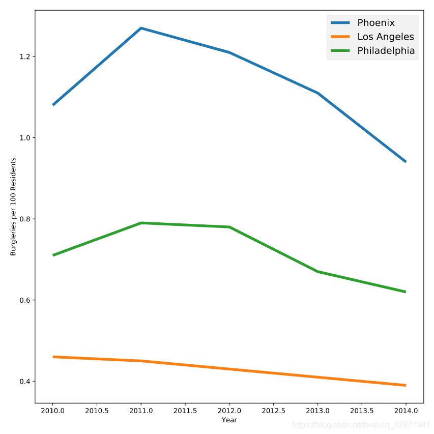
plt.style.use('ggplot')
plt.plot(data["Year"], data["Phoenix Police Dept"], label="Phoenix")
plt.plot(data["Year"], data["Los Angeles Police Dept"], label="Los Angeles")
plt.plot(data["Year"], data["Philadelphia Police Dept"], label="Philadelphia")
plt.legend()
plt.show()
print(plt.style.available)
['seaborn-bright', 'seaborn-deep', 'seaborn-whitegrid', '_classic_test', 'seaborn-poster', 'classic', 'seaborn-muted', 'fivethirtyeight', 'seaborn', 'seaborn-colorblind', 'fast', 'Solarize_Light2', 'seaborn-talk', 'dark_background', 'grayscale', 'seaborn-notebook', 'seaborn-darkgrid', 'seaborn-paper', 'seaborn-dark-palette', 'ggplot', 'seaborn-ticks', 'seaborn-white', 'bmh', 'tableau-colorblind10', 'seaborn-pastel', 'seaborn-dark']
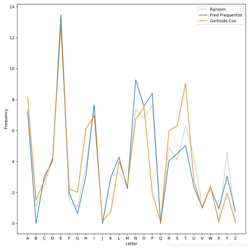
9. Identifying Bayes’ kidnapper 确认绑架Bayes的绑匪
The kidnapper left a long ransom note containing several unusual phrases. Help DataCamp by using a line plot to compare the frequency of letters in the ransom note to samples from the two main suspects.
绑架者留下了一封长长的勒索信,信中有几句不寻常的话。使用折线图将勒索信的频率与两名主要嫌疑人的样本进行比较。
plt.plot(ransom.letter, ransom.frequency,
         label='Ransom', linestyle=':', color='gray')
plt.plot(suspect1.letter, suspect1.frequency, label='Fred Frequentist')
plt.plot(suspect2.letter, suspect2.frequency, label='Gertrude Cox')
plt.xlabel("Letter")
plt.ylabel("Frequency")
plt.legend()
plt.show()
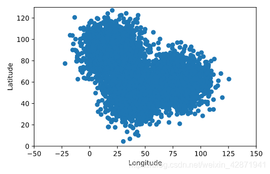
We know that Freddy Frequentist is the one who kidnapped Bayes the Golden Retriever. Now we need to learn where he is hiding.Our friends at the police station have acquired cell phone data, which gives some of Freddie’s locations over the past three weeks.
我们已经知道Freddy Frequentist就是绑架Bayes的人。现在我们需要知道他藏在哪里。我们在警察局的朋友已经获得了手机数据,这些数据显示了过去三周Freddy的一些位置。
print(cellphone.head())
   Unnamed: 0          x          y
0           0  28.136519  39.358650
1           1  44.642131  58.214270
2           2  34.921629  42.039109
3           3  31.034296  38.283153
4           4  36.419871  65.971441
plt.scatter(cellphone.x, cellphone.y)
plt.ylabel('Latitude')
plt.xlabel('Longitude')
plt.show()
We’ve done some magic so that the plot will appear over a map of our town. We can change the colors, markers, and transparency of the scatter plot.
我们让这些散点显示在了我们城镇的地图上,通过改变颜色,形状和透明度优化图表。
plt.scatter(cellphone.x, cellphone.y,
           color='red',
           marker='s', # marker style
           alpha=0.1) # 透明度
plt.ylabel('Latitude')
plt.xlabel('Longitude')
plt.show()

10. the average number of hours 警官工作的平均时长
Officer Deshaun wants to plot the average number of hours worked per week for him and his coworkers.
Deshaun警官想要画出他和他的同事每周工作的平均小时数。
print(hours)
   officer  avg_hours_worked  std_hours_worked
0  Deshaun                45                 3
1  Mengfei                33                 9
2   Aditya                42                 5
plt.bar(hours.officer, hours.avg_hours_worked,
        yerr=hours.std_hours_worked) # 误差线
plt.show()

Officer Deshaun has split out the average hours worked per week into desk_work and field_work.
Deshaun警官想把平均工作时间进一步细化,他把每周的平均工作时间分为案头工作和现场工作。
plt.bar(hours.officer, hours.desk_work, label='Desk Work')
plt.bar(hours.officer, hours.field_work, bottom=hours.desk_work, label='Field Work')
plt.legend()
plt.show()

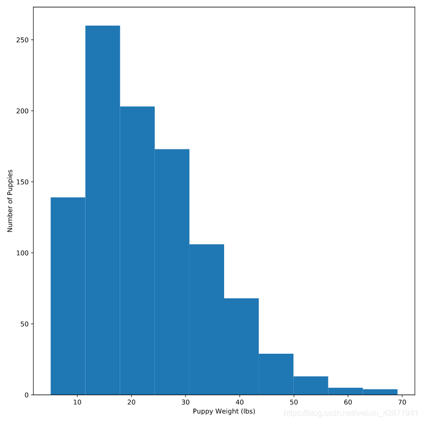
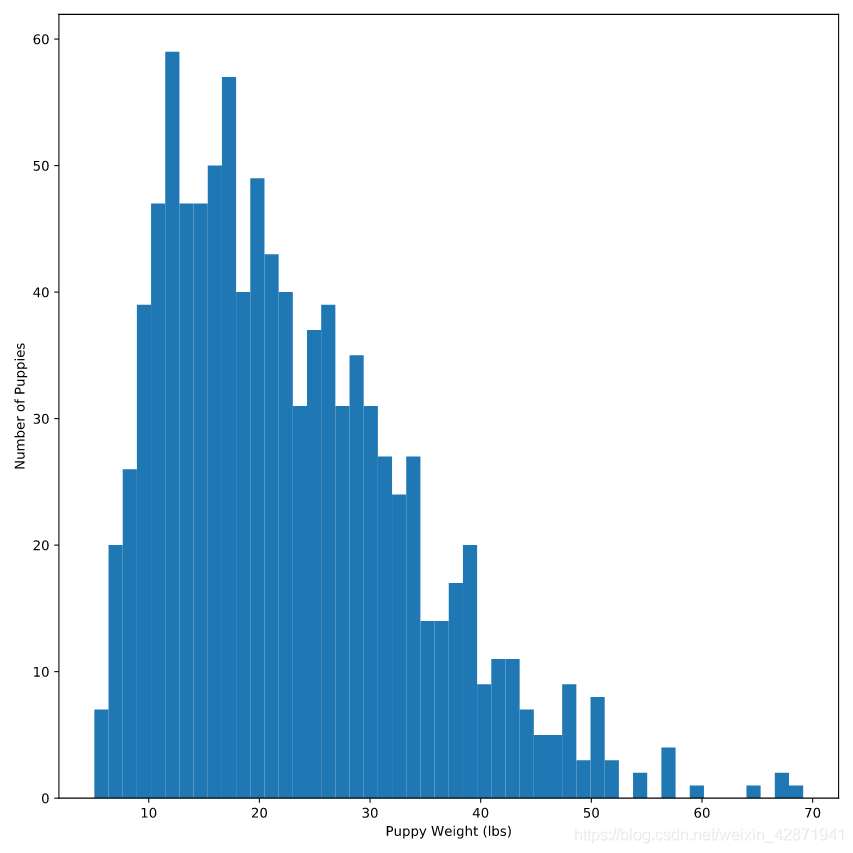
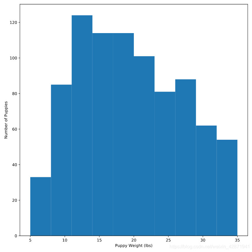
Modifying histograms
修改直方图
plt.hist(puppies.weight)
plt.xlabel('Puppy Weight (lbs)')
plt.ylabel('Number of Puppies')
plt.show()
plt.hist(puppies.weight,
        bins=50) # 箱子默认为10
plt.xlabel('Puppy Weight (lbs)')
plt.ylabel('Number of Puppies')
plt.show()
plt.hist(puppies.weight,
        range=(5, 35)) # 纵坐标区间修改
plt.xlabel('Puppy Weight (lbs)')
plt.ylabel('Number of Puppies')
plt.show()
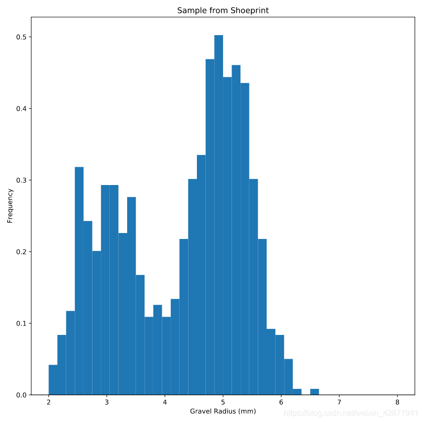
11. Where Fred is hiding Bayes 查找Bayes被藏位置
A shoe print at the crime scene contains a specific type of gravel. Based on the distribution of gravel radii, we can determine where the kidnapper recently visited.
犯罪现场的鞋印包含一种特殊类型的砾石。根据砾石的半径分布,我们可以确定绑架者最近去过的地方。
plt.hist(gravel.radius,
         bins=40,
         range=(2, 8),
         density=True)
plt.xlabel('Gravel Radius (mm)')
plt.ylabel('Frequency')
plt.title('Sample from Shoeprint')
plt.show()