高斯分布的乘积

假设有两个高斯分布：

$$p_1(x) = (2\pi\sigma_1^2)^{-\frac{1}{2}}exp\{ -\frac{1}{2} \frac{(x-\mu_1)^2}{\sigma_1^2} \}$$ $$p_2(x) = (2\pi\sigma_2^2)^{-\frac{1}{2}}exp\{ -\frac{1}{2} \frac{(x-\mu_2)^2}{\sigma_2^2}$$

高斯分布相乘

计算这两个高斯分布的乘积:

$$p_1(x)p_2(x) = \frac{1}{2\pi \sqrt{\sigma_1^2\sigma_2^2} }exp\{ -\{ \frac{(x-\mu_1)^2}{2\sigma_1^2} + \frac{(x-\mu_2)^2}{2\sigma_2^2} \} \}$$
高斯分布的乘积还是高斯分布，且根据这篇博客 直观理解高斯相乘可以计算出 $p_1(x)p_2(x)$的均值 $\mu$和方差 $\sigma$。
$$\mu = \frac{\mu_1 \sigma_2^2 + \mu_2 \sigma_1^2}{ \sigma_1^2+\sigma_2^2}$$ $$\frac{1}{\sigma^2} = \frac{1}{\sigma_1^2}+\frac{1}{\sigma_2^2}$$ $$\sigma^2 = \frac{\sigma_1^2\sigma_2^2}{\sigma_1^2+\sigma_2^2}$$
接下来分析一下 $\mu$和 $\sigma^2$
首先是均值 $\mu$
$$\mu - \mu_1 =\frac{\mu_1 \sigma_2^2 + \mu_2 \sigma_1^2}{ \sigma_1^2+\sigma_2^2} -\frac{\mu_1 \sigma_1^2 + \mu_1\sigma_2^2}{\sigma_1^2+\sigma_2^2} =\frac{(\mu_2-\mu_1)\sigma_1^2}{\sigma_1^2+\sigma_2^2}$$ $$\mu - \mu_2 =\frac{\mu_1 \sigma_2^2 + \mu_2 \sigma_1^2}{ \sigma_1^2+\sigma_2^2} -\frac{\mu_2 \sigma_1^2 + \mu_2\sigma_2^2}{\sigma_1^2+\sigma_2^2} =\frac{(\mu_1-\mu_2)\sigma_2^2}{\sigma_1^2+\sigma_2^2}$$
当 $\mu_1>\mu_2$时：
$\mu-\mu_1<0, \mu-\mu_2>0$ 所以， $\mu_2<\mu<\mu_1$
当 $\mu_1<\mu_2$时：
$\mu-\mu_1>0, \mu-\mu_2<0$ 所以， $\mu_1<\mu<\mu_2$
当 $\mu_1=\mu_2$时：
$\mu-\mu_1=0, \mu-\mu_2=0$ 所以， $\mu_1=\mu=\mu_2$
可以看出 $\mu$是位于 $\mu_1$和 $\mu_2$之间。

接下来是方差$\sigma$

$$\sigma^2-\sigma_1^2 = \frac{\sigma_1^2\sigma_2^2}{\sigma_1^2+\sigma_2^2}-\sigma_1^2=\frac{-\sigma_1^4}{\sigma_1^2+\sigma_2^2}<0$$ $$\sigma^2-\sigma_2^2 = \frac{\sigma_1^2\sigma_2^2}{\sigma_1^2+\sigma_2^2}-\sigma_2^2=\frac{-\sigma_2^4}{\sigma_1^2+\sigma_2^2}<0$$
所以 $p_1(x)p_2(x)$的方差比 $p_1(x)$和 $p_2(x)$的方差都要小。

代码验证高斯分布相乘

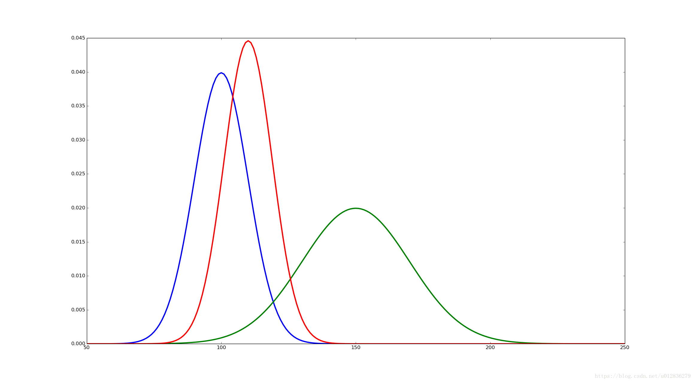
紧接着，通过python代码验证这个结果：
其中，红色的曲线表示高斯分布的乘积，其详细的代码如下所示：

import matplotlib.pyplot as plt
from math import *

class Distribution:
    def __init__(self,mu,sigma,x,values,start,end):
        self.mu = mu
        self.sigma = sigma
        self.values = values
        self.x = x
        self.start = start
        self.end =end

    def normalize(self):
        s = float(sum(self.values))
        if s != 0.0:
            self.values = [i/s for i in self.values]

    def value(self, index):
        index -= self.start
        if index<0 or index >= len(self.values):
            return 0.0
        else:
            return self.values[index]

    @staticmethod
    def gaussian(mu,sigma,cut = 5.0):
        sigma2 = sigma*sigma
        extent = int(ceil(cut*sigma))
        values = []
        x_lim=[]
        for x in xrange(mu-extent,mu+extent+1):
            x_lim.append(x)
            values.append(exp((-0.5*(x-mu)*(x-mu))/sigma2))
        p1=Distribution(mu,sigma,x_lim,values,mu-extent,mu-extent+len(values))
        p1.normalize()
        return p1

if __name__=='__main__':
    p1 = Distribution.gaussian(100,10)
    plt.plot(p1.x,p1.values,"b-",linewidth=3)

    p2 = Distribution.gaussian(150,20)
    plt.plot(p2.x,p2.values,"g-",linewidth=3)

    start = min(p1.start,p2.start)
    end = max(p1.end,p2.end)
    mul_dist = []
    x_lim = []

    for index in range(start,end):
        x_lim.append(index)
        mul_dist.append(p1.value(index)*p2.value(index))
    #normalize the distribution
    s= float(sum(mul_dist))
    if s!=0.0:
        mul_dist=[i/s for i in mul_dist]

    plt.plot(x_lim,mul_dist,"r-",linewidth=3)
    plt.show()