最近在kaggle上找项目练习,发现一个 TMDB电影票房预测项目比较适合练手。这里记录在下。
目标是通过train集中的数据训练模型,将test集数据导入模型得出目标值revenue即票房,上传结果得到分数和排名。
数据可以从kaggle网站上直接下载,文中用到的额外数据可从
https://www.kaggle.com/kamalchhirang/tmdb-competition-additional-features
和
https://www.kaggle.com/kamalchhirang/tmdb-box-office-prediction-more-training-data
下载。
EDA
train.info()
载入数据并整理后大体观察
<class 'pandas.core.frame.DataFrame'>
Int64Index: 3000 entries, 0 to 2999
Data columns (total 53 columns):
id                       3000 non-null int64
belongs_to_collection    604 non-null object
budget                   3000 non-null int64
genres                   3000 non-null object
homepage                 946 non-null object
imdb_id                  3000 non-null object
original_language        3000 non-null object
original_title           3000 non-null object
overview                 2992 non-null object
popularity               3000 non-null float64
poster_path              2999 non-null object
production_companies     2844 non-null object
production_countries     2945 non-null object
release_date             3000 non-null object
runtime                  2998 non-null float64
spoken_languages         2980 non-null object
status                   3000 non-null object
tagline                  2403 non-null object
title                    3000 non-null object
Keywords                 2724 non-null object
cast                     2987 non-null object
crew                     2984 non-null object
revenue                  3000 non-null int64
logRevenue               3000 non-null float64
release_month            3000 non-null int32
release_day              3000 non-null int32
release_year             3000 non-null int32
release_dayofweek        3000 non-null int64
release_quarter          3000 non-null int64
Action                   3000 non-null int64
Adventure                3000 non-null int64
Animation                3000 non-null int64
Comedy                   3000 non-null int64
Crime                    3000 non-null int64
Documentary              3000 non-null int64
Drama                    3000 non-null int64
Family                   3000 non-null int64
Fantasy                  3000 non-null int64
Foreign                  3000 non-null int64
History                  3000 non-null int64
Horror                   3000 non-null int64
Music                    3000 non-null int64
Mystery                  3000 non-null int64
Romance                  3000 non-null int64
Science Fiction          3000 non-null int64
TV Movie                 3000 non-null int64
Thriller                 3000 non-null int64
War                      3000 non-null int64
Western                  3000 non-null int64
popularity2              2882 non-null float64
rating                   3000 non-null float64
totalVotes               3000 non-null float64
meanRevenueByRating      8 non-null float64
dtypes: float64(7), int32(3), int64(25), object(18)
memory usage: 1.2+ MB
主要的几项特征:
- budget:预算
- revenue:票房
- rating:观众打分
- totalVotes:观众打分数量
- popularity:流行系数(怎么得出的暂未可知)
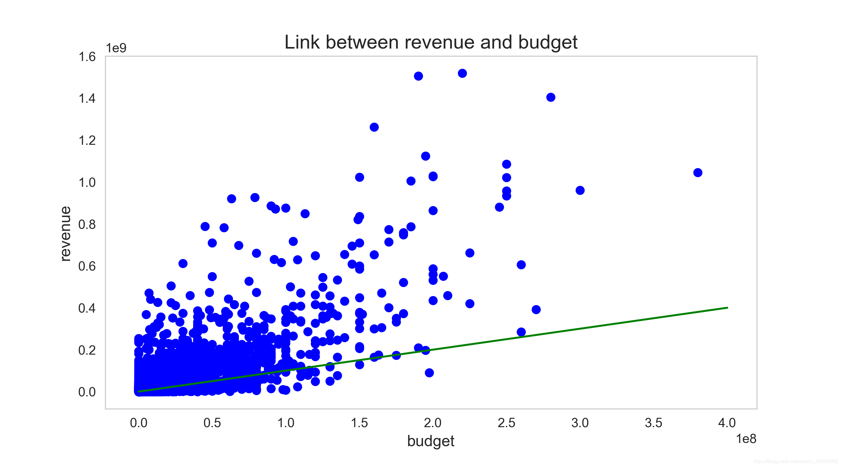
票房和预算呈较明显的正相关关系。这很符合常识,但也不定,现在也挺多投资高票房低的烂片的。
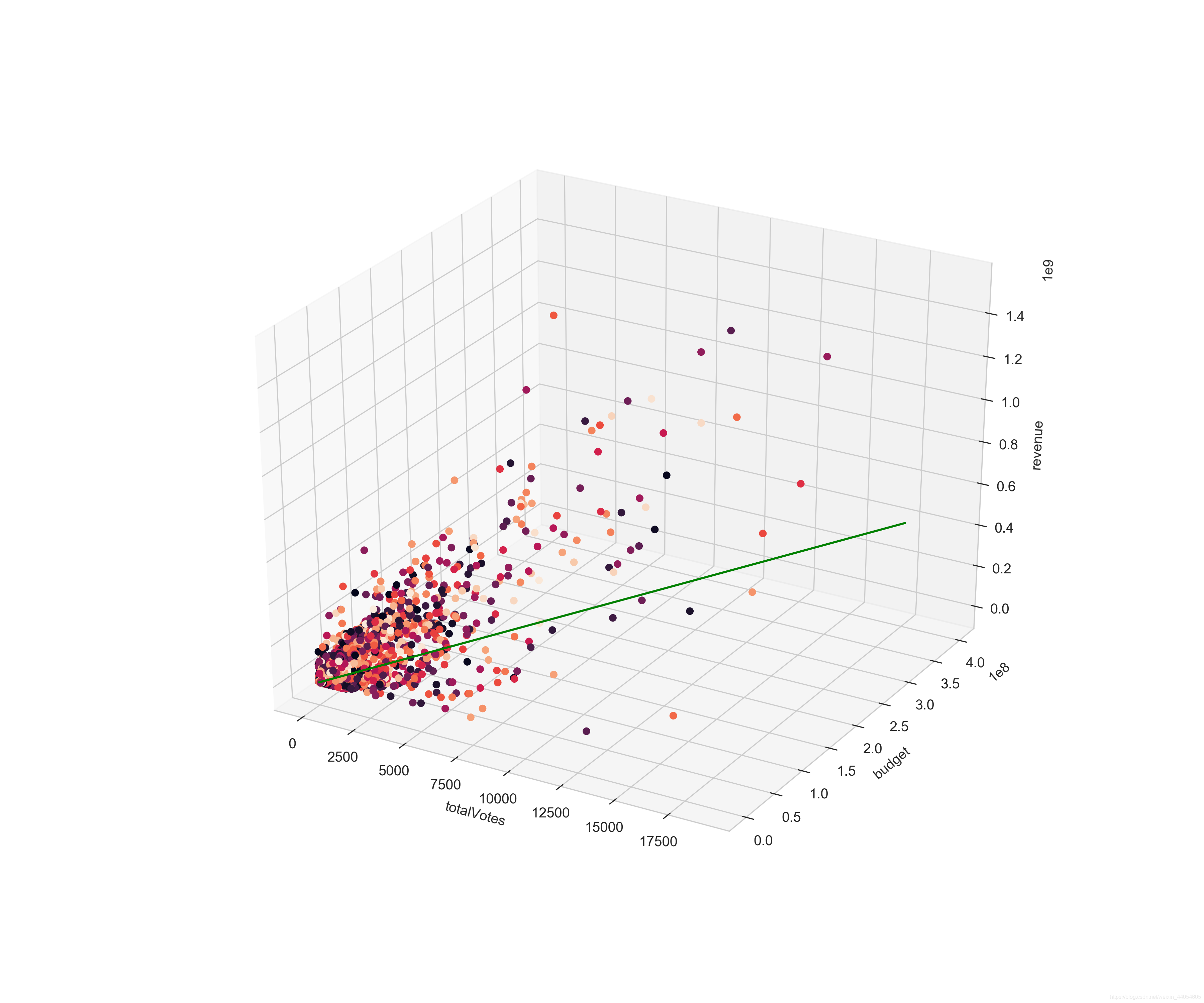
除了预算外,票房和观众打分数量也有一定关系。这也符合常识,不管观众打分高低,只要有大量观众打分,就说明该电影是舆论热点,票房就不会太低。
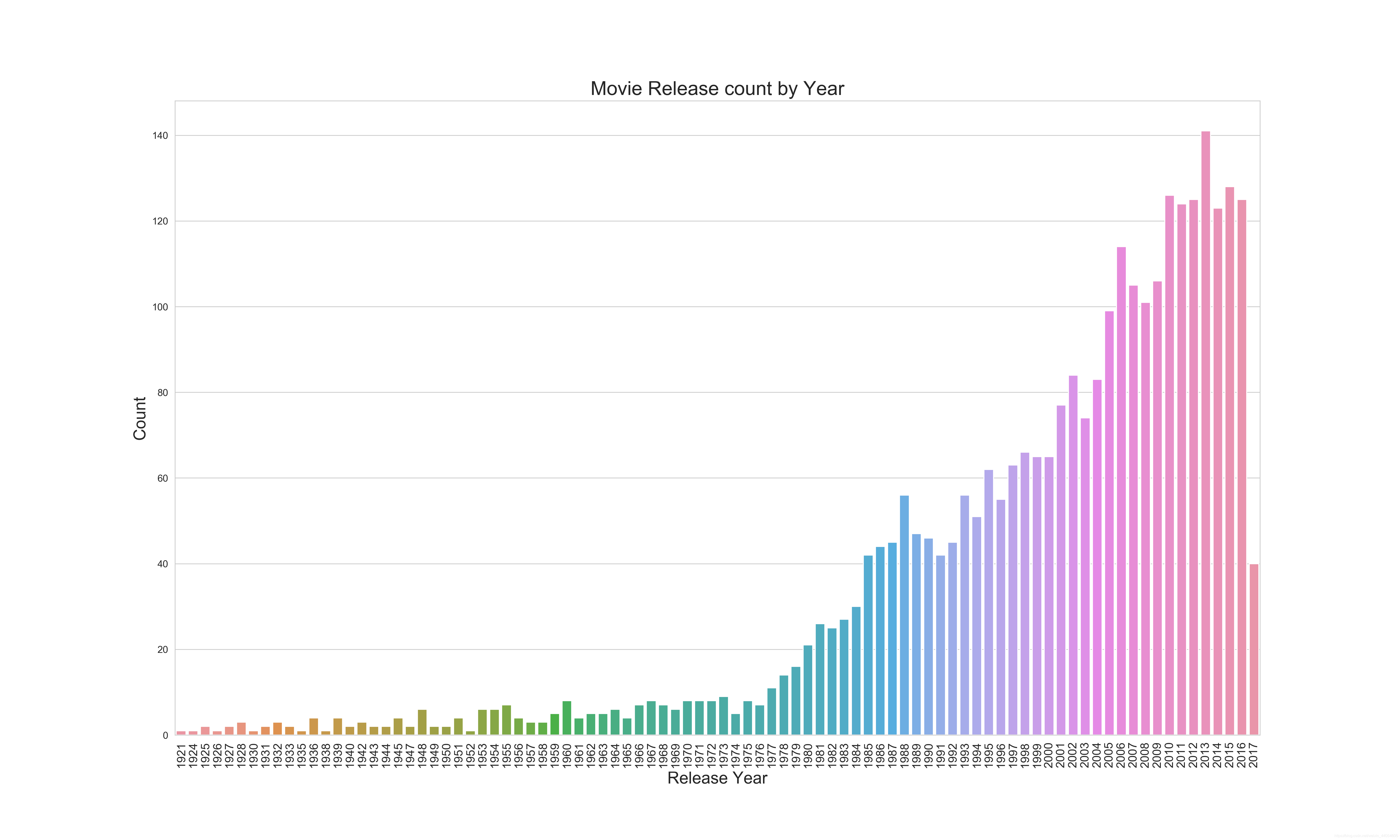
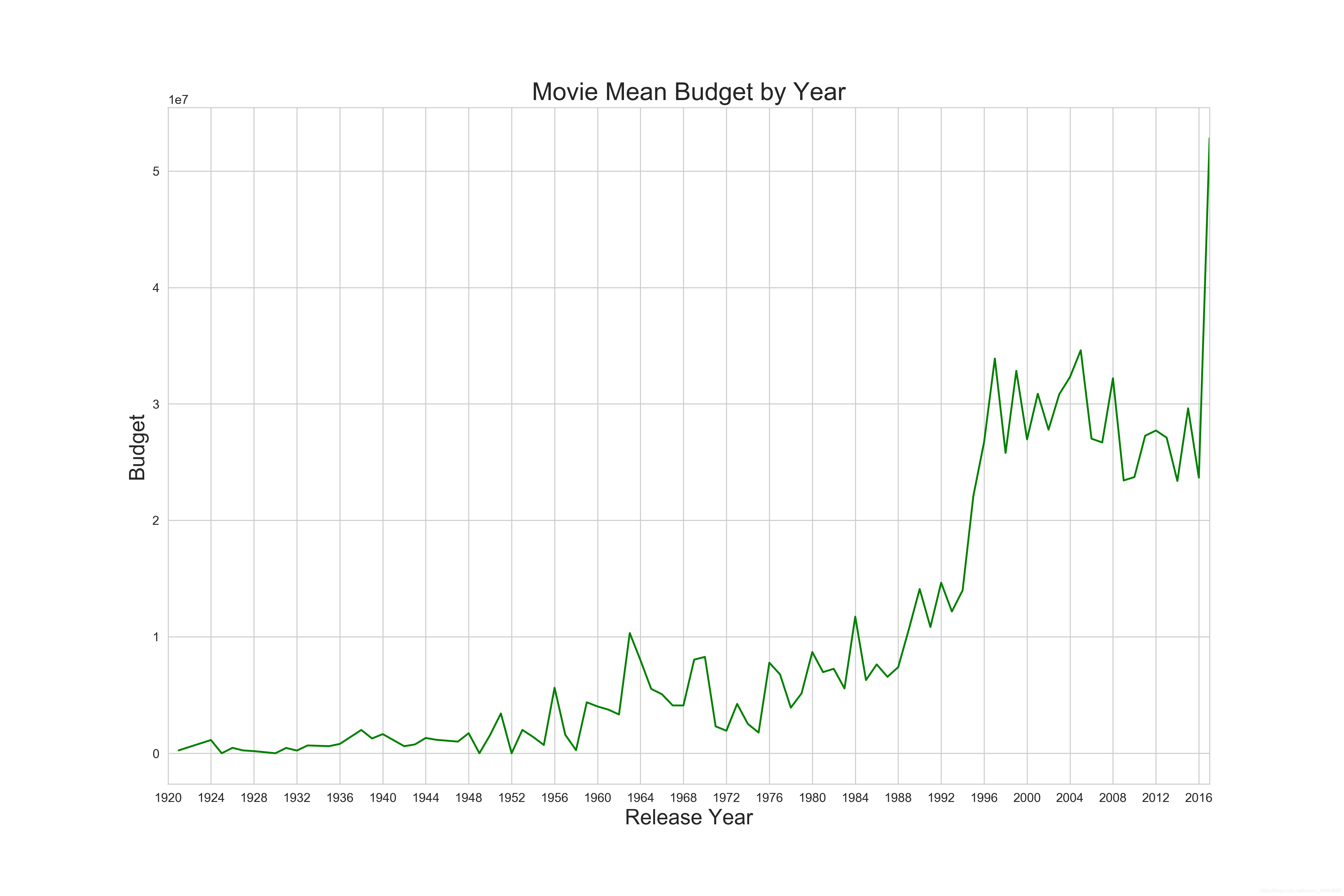
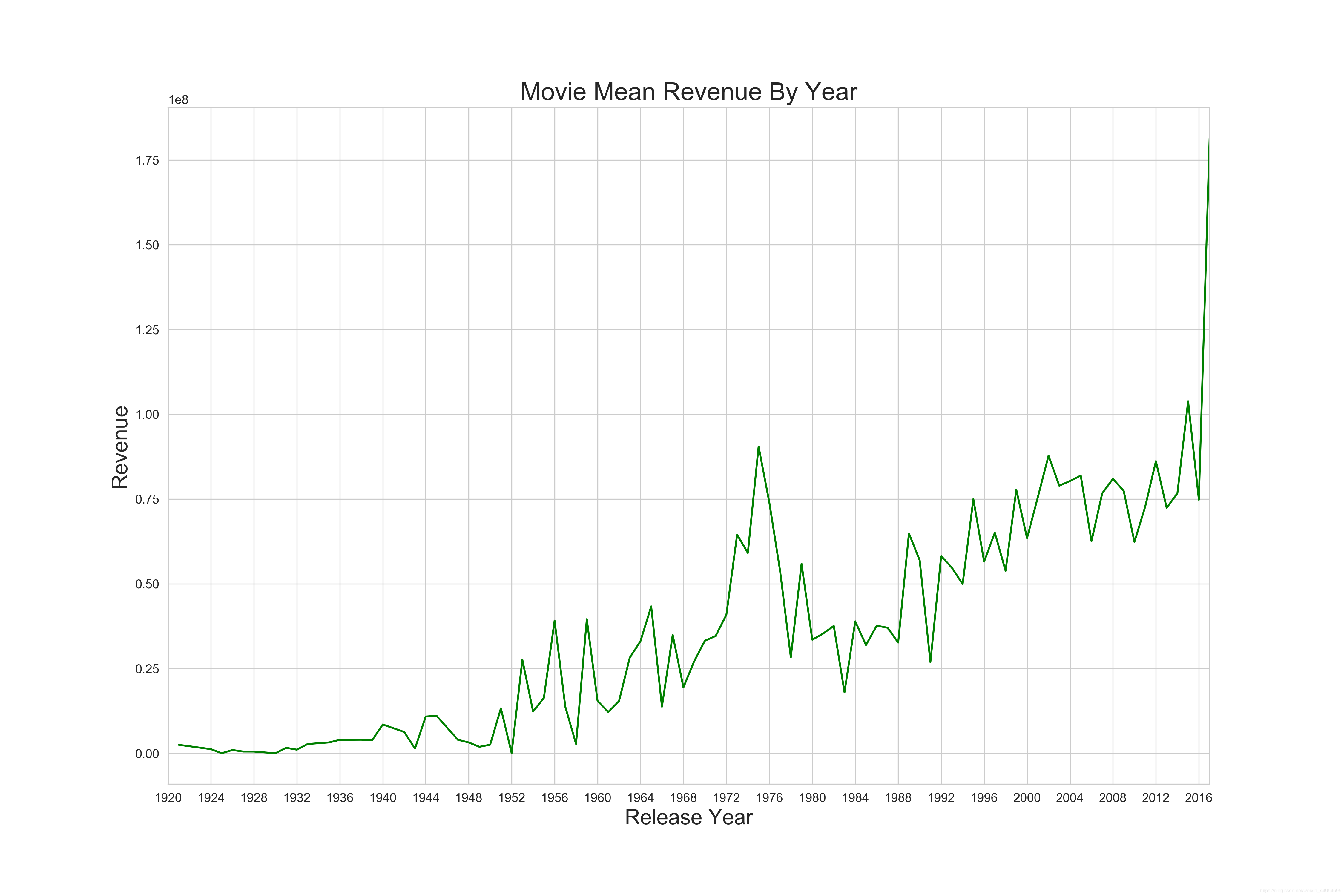
近几年的电影市场无论是投资还是票房都有比较大的增长,说明了电影市场的火爆。也提醒我们后续的特征工程需要关注电影上映年份。
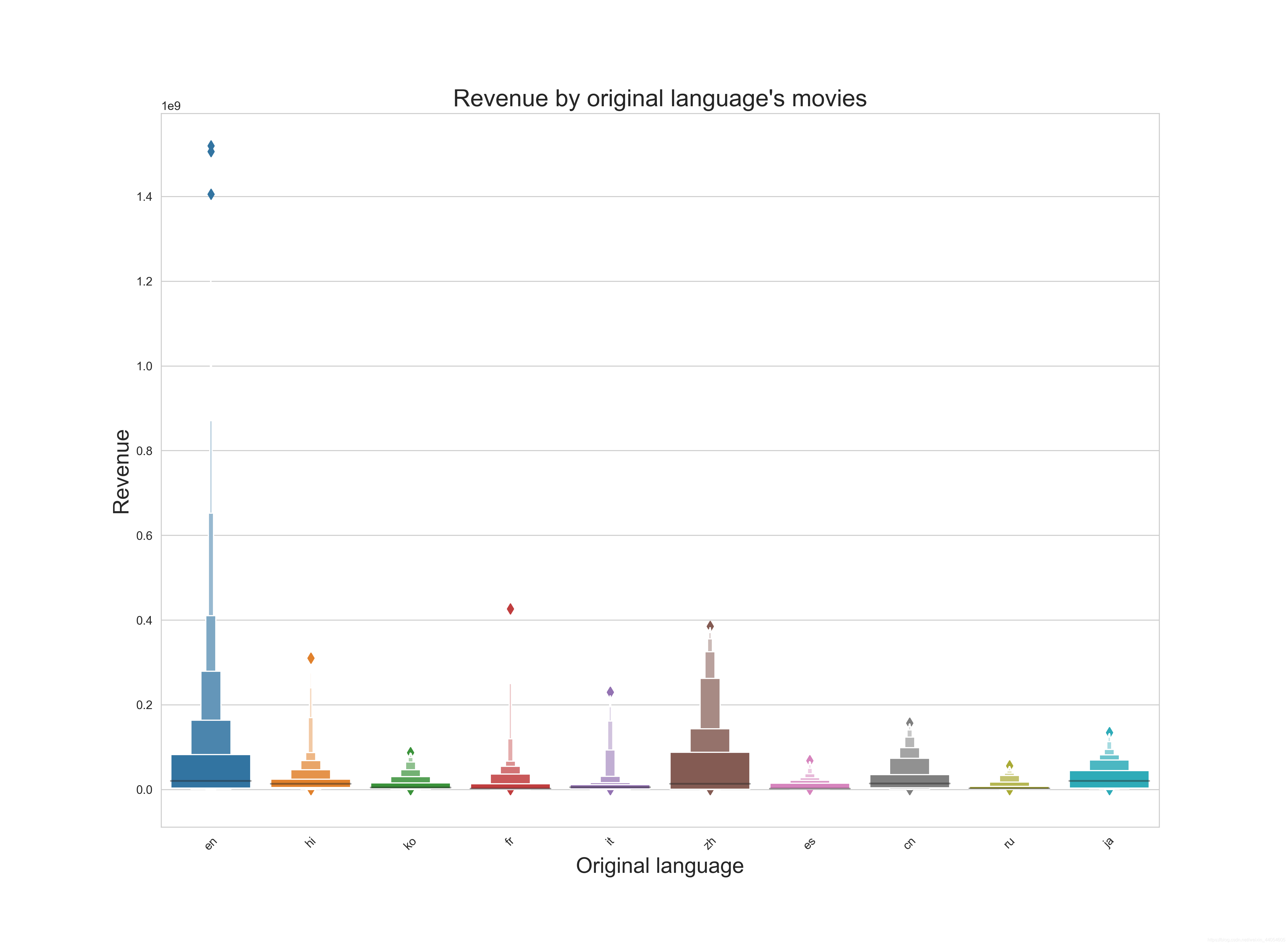
通过电影的语言来看票房。en表示英语。毕竟世界语言,无论是票房的体量还是高票房爆款,都独占鳌头。zh就是你心里想的那个,中文。可见华语电影对于english可以望其项背了。语言对票房也有一定反映。
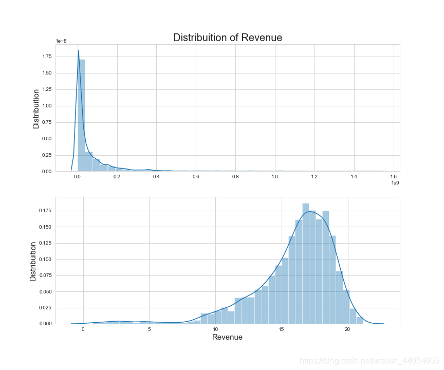
票房的分布明显右偏,可以通过np.logp1方法转换为对数形式实现数据的正态化,但记得在得到最后的预测数据后再用np.expm1方法转换回来。
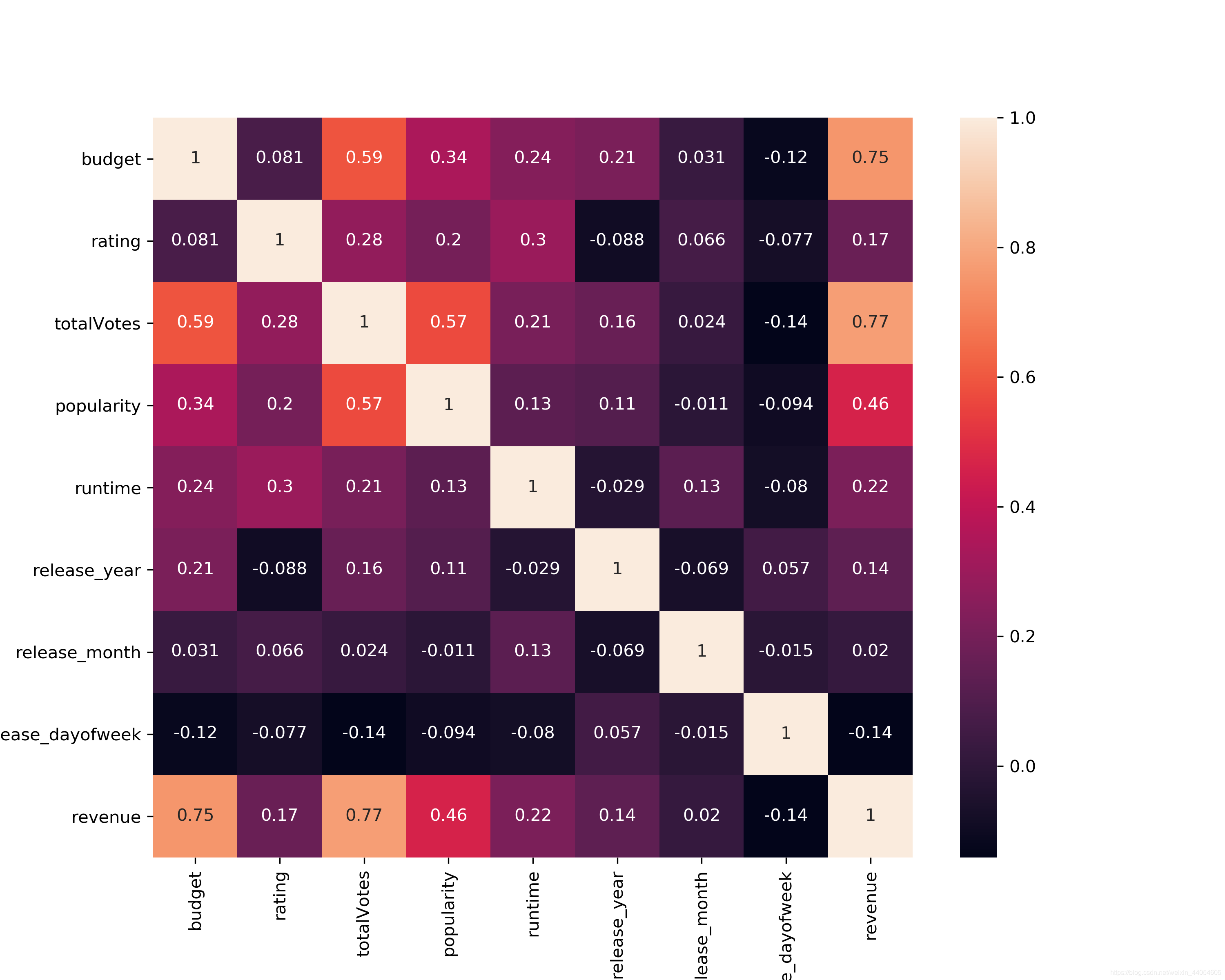
通过热力图观察几个主要特征跟票房的皮尔逊系数(线性相关系数),及其彼此的系数。可见跟票房revenue最相关的为budget,totalVotes,popularity。
特征工程
特征工程太过繁琐,不一一叙述,直接上整体代码。
import numpy as np
import pandas as pd
import warnings
from tqdm import tqdm
from sklearn.preprocessing import LabelEncoder
warnings.filterwarnings("ignore")

def prepare(df):
    global json_cols
    global train_dict
    df['rating'] = df['rating'].fillna(1.5)
    df['totalVotes'] = df['totalVotes'].fillna(6)
    df['weightedRating'] = (df['rating'] * df['totalVotes'] + 6.367 * 300) / (df['totalVotes'] + 300)

    df[['release_month', 'release_day', 'release_year']] = df['release_date'].str.split('/', expand=True).replace(
        np.nan, 0).astype(int)
    df['release_year'] = df['release_year']
    df.loc[(df['release_year'] <= 19) & (df['release_year'] < 100), "release_year"] += 2000
    df.loc[(df['release_year'] > 19) & (df['release_year'] < 100), "release_year"] += 1900

    releaseDate = pd.to_datetime(df['release_date'])
    df['release_dayofweek'] = releaseDate.dt.dayofweek
    df['release_quarter'] = releaseDate.dt.quarter

    df['originalBudget'] = df['budget']
    df['inflationBudget'] = df['budget'] + df['budget'] * 1.8 / 100 * (
                2018 - df['release_year'])  # Inflation simple formula
    df['budget'] = np.log1p(df['budget'])

    df['genders_0_crew'] = df['crew'].apply(lambda x: sum([1 for i in x if i['gender'] == 0]))
    df['genders_1_crew'] = df['crew'].apply(lambda x: sum([1 for i in x if i['gender'] == 1]))
    df['genders_2_crew'] = df['crew'].apply(lambda x: sum([1 for i in x if i['gender'] == 2]))
    df['_collection_name'] = df['belongs_to_collection'].apply(lambda x: x[0]['name'] if x != {} else '').fillna('')
    le = LabelEncoder()
    df['_collection_name'] = le.fit_transform(df['_collection_name'])
    df['_num_Keywords'] = df['Keywords'].apply(lambda x: len(x) if x != {} else 0)
    df['_num_cast'] = df['cast'].apply(lambda x: len(x) if x != {} else 0)

    df['_popularity_mean_year'] = df['popularity'] / df.groupby("release_year")["popularity"].transform('mean')
    df['_budget_runtime_ratio'] = df['budget'] / df['runtime']
    df['_budget_popularity_ratio'] = df['budget'] / df['popularity']
    df['_budget_year_ratio'] = df['budget'] / (df['release_year'] * df['release_year'])
    df['_releaseYear_popularity_ratio'] = df['release_year'] / df['popularity']
    df['_releaseYear_popularity_ratio2'] = df['popularity'] / df['release_year']

    df['_popularity_totalVotes_ratio'] = df['totalVotes'] / df['popularity']
    df['_rating_popularity_ratio'] = df['rating'] / df['popularity']
    df['_rating_totalVotes_ratio'] = df['totalVotes'] / df['rating']
    df['_totalVotes_releaseYear_ratio'] = df['totalVotes'] / df['release_year']
    df['_budget_rating_ratio'] = df['budget'] / df['rating']
    df['_runtime_rating_ratio'] = df['runtime'] / df['rating']
    df['_budget_totalVotes_ratio'] = df['budget'] / df['totalVotes']

    df['has_homepage'] = 1
    df.loc[pd.isnull(df['homepage']), "has_homepage"] = 0

    df['isbelongs_to_collectionNA'] = 0
    df.loc[pd.isnull(df['belongs_to_collection']), "isbelongs_to_collectionNA"] = 1

    df['isTaglineNA'] = 0
    df.loc[df['tagline'] == 0, "isTaglineNA"] = 1

    df['isOriginalLanguageEng'] = 0
    df.loc[df['original_language'] == "en", "isOriginalLanguageEng"] = 1

    df['isTitleDifferent'] = 1
    df.loc[df['original_title'] == df['title'], "isTitleDifferent"] = 0

    df['isMovieReleased'] = 1
    df.loc[df['status'] != "Released", "isMovieReleased"] = 0

    # get collection id
    df['collection_id'] = df['belongs_to_collection'].apply(lambda x: np.nan if len(x) == 0 else x[0]['id'])

    df['original_title_letter_count'] = df['original_title'].str.len()
    df['original_title_word_count'] = df['original_title'].str.split().str.len()

    df['title_word_count'] = df['title'].str.split().str.len()
    df['overview_word_count'] = df['overview'].str.split().str.len()
    df['tagline_word_count'] = df['tagline'].str.split().str.len()

    df['production_countries_count'] = df['production_countries'].apply(lambda x: len(x))
    df['production_companies_count'] = df['production_companies'].apply(lambda x: len(x))
    df['crew_count'] = df['crew'].apply(lambda x: len(x) if x != {} else 0)

    # df['meanruntimeByYear'] = df.groupby("release_year")["runtime"].aggregate('mean')
    # df['meanPopularityByYear'] = df.groupby("release_year")["popularity"].aggregate('mean')
    # df['meanBudgetByYear'] = df.groupby("release_year")["budget"].aggregate('mean')
    # df['meantotalVotesByYear'] = df.groupby("release_year")["totalVotes"].aggregate('mean')
    # df['meanTotalVotesByRating'] = df.groupby("rating")["totalVotes"].aggregate('mean')
    # df['medianBudgetByYear'] = df.groupby("release_year")["budget"].aggregate('median')

    for col in ['genres', 'production_countries', 'spoken_languages', 'production_companies']:
        df[col] = df[col].map(lambda x: sorted(
            list(set([n if n in train_dict[col] else col + '_etc' for n in [d['name'] for d in x]]))))\
            .map(lambda x: ','.join(map(str, x)))
        temp = df[col].str.get_dummies(sep=',')
        df = pd.concat([df, temp], axis=1, sort=False)
    df.drop(['genres_etc'], axis=1, inplace=True)

    df = df.drop(['id', 'revenue', 'belongs_to_collection', 'genres', 'homepage', 'imdb_id', 'overview', 'runtime'
                     , 'poster_path', 'production_companies', 'production_countries', 'release_date', 'spoken_languages'
                     , 'status', 'title', 'Keywords', 'cast', 'crew', 'original_language', 'original_title', 'tagline',
                  'collection_id'
                  ], axis=1)

    df.fillna(value=0.0, inplace=True)
    return df


def get_dictionary(s):
    try:
        d = eval(s)
    except:
        d = {}
    return d


def get_json_dict(df) :
    global json_cols
    result = dict()
    for e_col in json_cols :
        d = dict()
        rows = df[e_col].values
        for row in rows :
            if row is None : continue
            for i in row :
                if i['name'] not in d :
                    d[i['name']] = 0
                d[i['name']] += 1
        result[e_col] = d
    return result


if __name__ == '__main__':
    train = pd.read_csv('./train.csv')
    train.loc[train['id'] == 16, 'revenue'] = 192864  # Skinning
    train.loc[train['id'] == 90, 'budget'] = 30000000  # Sommersby
    train.loc[train['id'] == 118, 'budget'] = 60000000  # Wild Hogs
    train.loc[train['id'] == 149, 'budget'] = 18000000  # Beethoven
    train.loc[train['id'] == 313, 'revenue'] = 12000000  # The Cookout
    train.loc[train['id'] == 451, 'revenue'] = 12000000  # Chasing Liberty
    train.loc[train['id'] == 464, 'budget'] = 20000000  # Parenthood
    train.loc[train['id'] == 470, 'budget'] = 13000000  # The Karate Kid, Part II
    train.loc[train['id'] == 513, 'budget'] = 930000  # From Prada to Nada
    train.loc[train['id'] == 797, 'budget'] = 8000000  # Welcome to Dongmakgol
    train.loc[train['id'] == 819, 'budget'] = 90000000  # Alvin and the Chipmunks: The Road Chip
    train.loc[train['id'] == 850, 'budget'] = 90000000  # Modern Times
    train.loc[train['id'] == 1007, 'budget'] = 2  # Zyzzyx Road
    train.loc[train['id'] == 1112, 'budget'] = 7500000  # An Officer and a Gentleman
    train.loc[train['id'] == 1131, 'budget'] = 4300000  # Smokey and the Bandit
    train.loc[train['id'] == 1359, 'budget'] = 10000000  # Stir Crazy
    train.loc[train['id'] == 1542, 'budget'] = 1  # All at Once
    train.loc[train['id'] == 1570, 'budget'] = 15800000  # Crocodile Dundee II
    train.loc[train['id'] == 1571, 'budget'] = 4000000  # Lady and the Tramp
    train.loc[train['id'] == 1714, 'budget'] = 46000000  # The Recruit
    train.loc[train['id'] == 1721, 'budget'] = 17500000  # Cocoon
    train.loc[train['id'] == 1865, 'revenue'] = 25000000  # Scooby-Doo 2: Monsters Unleashed
    train.loc[train['id'] == 1885, 'budget'] = 12  # In the Cut
    train.loc[train['id'] == 2091, 'budget'] = 10  # Deadfall
    train.loc[train['id'] == 2268, 'budget'] = 17500000  # Madea Goes to Jail budget
    train.loc[train['id'] == 2491, 'budget'] = 6  # Never Talk to Strangers
    train.loc[train['id'] == 2602, 'budget'] = 31000000  # Mr. Holland's Opus
    train.loc[train['id'] == 2612, 'budget'] = 15000000  # Field of Dreams
    train.loc[train['id'] == 2696, 'budget'] = 10000000  # Nurse 3-D
    train.loc[train['id'] == 2801, 'budget'] = 10000000  # Fracture
    train.loc[train['id'] == 335, 'budget'] = 2
    train.loc[train['id'] == 348, 'budget'] = 12
    train.loc[train['id'] == 470, 'budget'] = 13000000
    train.loc[train['id'] == 513, 'budget'] = 1100000
    train.loc[train['id'] == 640, 'budget'] = 6
    train.loc[train['id'] == 696, 'budget'] = 1
    train.loc[train['id'] == 797, 'budget'] = 8000000
    train.loc[train['id'] == 850, 'budget'] = 1500000
    train.loc[train['id'] == 1199, 'budget'] = 5
    train.loc[train['id'] == 1282, 'budget'] = 9  # Death at a Funeral
    train.loc[train['id'] == 1347, 'budget'] = 1
    train.loc[train['id'] == 1755, 'budget'] = 2
    train.loc[train['id'] == 1801, 'budget'] = 5
    train.loc[train['id'] == 1918, 'budget'] = 592
    train.loc[train['id'] == 2033, 'budget'] = 4
    train.loc[train['id'] == 2118, 'budget'] = 344
    train.loc[train['id'] == 2252, 'budget'] = 130
    train.loc[train['id'] == 2256, 'budget'] = 1
    train.loc[train['id'] == 2696, 'budget'] = 10000000

    test = pd.read_csv('./test.csv')

    # Clean Data
    test.loc[test['id'] == 6733, 'budget'] = 5000000
    test.loc[test['id'] == 3889, 'budget'] = 15000000
    test.loc[test['id'] == 6683, 'budget'] = 50000000
    test.loc[test['id'] == 5704, 'budget'] = 4300000
    test.loc[test['id'] == 6109, 'budget'] = 281756
    test.loc[test['id'] == 7242, 'budget'] = 10000000
    test.loc[test['id'] == 7021, 'budget'] = 17540562  # Two Is a Family
    test.loc[test['id'] == 5591, 'budget'] = 4000000  # The Orphanage
    test.loc[test['id'] == 4282, 'budget'] = 20000000  # Big Top Pee-wee
    test.loc[test['id'] == 3033, 'budget'] = 250
    test.loc[test['id'] == 3051, 'budget'] = 50
    test.loc[test['id'] == 3084, 'budget'] = 337
    test.loc[test['id'] == 3224, 'budget'] = 4
    test.loc[test['id'] == 3594, 'budget'] = 25
    test.loc[test['id'] == 3619, 'budget'] = 500
    test.loc[test['id'] == 3831, 'budget'] = 3
    test.loc[test['id'] == 3935, 'budget'] = 500
    test.loc[test['id'] == 4049, 'budget'] = 995946
    test.loc[test['id'] == 4424, 'budget'] = 3
    test.loc[test['id'] == 4460, 'budget'] = 8
    test.loc[test['id'] == 4555, 'budget'] = 1200000
    test.loc[test['id'] == 4624, 'budget'] = 30
    test.loc[test['id'] == 4645, 'budget'] = 500
    test.loc[test['id'] == 4709, 'budget'] = 450
    test.loc[test['id'] == 4839, 'budget'] = 7
    test.loc[test['id'] == 3125, 'budget'] = 25
    test.loc[test['id'] == 3142, 'budget'] = 1
    test.loc[test['id'] == 3201, 'budget'] = 450
    test.loc[test['id'] == 3222, 'budget'] = 6
    test.loc[test['id'] == 3545, 'budget'] = 38
    test.loc[test['id'] == 3670, 'budget'] = 18
    test.loc[test['id'] == 3792, 'budget'] = 19
    test.loc[test['id'] == 3881, 'budget'] = 7
    test.loc[test['id'] == 3969, 'budget'] = 400
    test.loc[test['id'] == 4196, 'budget'] = 6
    test.loc[test['id'] == 4221, 'budget'] = 11
    test.loc[test['id'] == 4222, 'budget'] = 500
    test.loc[test['id'] == 4285, 'budget'] = 11
    test.loc[test['id'] == 4319, 'budget'] = 1
    test.loc[test['id'] == 4639, 'budget'] = 10
    test.loc[test['id'] == 4719, 'budget'] = 45
    test.loc[test['id'] == 4822, 'budget'] = 22
    test.loc[test['id'] == 4829, 'budget'] = 20
    test.loc[test['id'] == 4969, 'budget'] = 20
    test.loc[test['id'] == 5021, 'budget'] = 40
    test.loc[test['id'] == 5035, 'budget'] = 1
    test.loc[test['id'] == 5063, 'budget'] = 14
    test.loc[test['id'] == 5119, 'budget'] = 2
    test.loc[test['id'] == 5214, 'budget'] = 30
    test.loc[test['id'] == 5221, 'budget'] = 50
    test.loc[test['id'] == 4903, 'budget'] = 15
    test.loc[test['id'] == 4983, 'budget'] = 3
    test.loc[test['id'] == 5102, 'budget'] = 28
    test.loc[test['id'] == 5217, 'budget'] = 75
    test.loc[test['id'] == 5224, 'budget'] = 3
    test.loc[test['id'] == 5469, 'budget'] = 20
    test.loc[test['id'] == 5840, 'budget'] = 1
    test.loc[test['id'] == 5960, 'budget'] = 30
    test.loc[test['id'] == 6506, 'budget'] = 11
    test.loc[test['id'] == 6553, 'budget'] = 280
    test.loc[test['id'] == 6561, 'budget'] = 7
    test.loc[test['id'] == 6582, 'budget'] = 218
    test.loc[test['id'] == 6638, 'budget'] = 5
    test.loc[test['id'] == 6749, 'budget'] = 8
    test.loc[test['id'] == 6759, 'budget'] = 50
    test.loc[test['id'] == 6856, 'budget'] = 10
    test.loc[test['id'] == 6858, 'budget'] = 100
    test.loc[test['id'] == 6876, 'budget'] = 250
    test.loc[test['id'] == 6972, 'budget'] = 1
    test.loc[test['id'] == 7079, 'budget'] = 8000000
    test.loc[test['id'] == 7150, 'budget'] = 118
    test.loc[test['id'] == 6506, 'budget'] = 118
    test.loc[test['id'] == 7225, 'budget'] = 6
    test.loc[test['id'] == 7231, 'budget'] = 85
    test.loc[test['id'] == 5222, 'budget'] = 5
    test.loc[test['id'] == 5322, 'budget'] = 90
    test.loc[test['id'] == 5350, 'budget'] = 70
    test.loc[test['id'] == 5378, 'budget'] = 10
    test.loc[test['id'] == 5545, 'budget'] = 80
    test.loc[test['id'] == 5810, 'budget'] = 8
    test.loc[test['id'] == 5926, 'budget'] = 300
    test.loc[test['id'] == 5927, 'budget'] = 4
    test.loc[test['id'] == 5986, 'budget'] = 1
    test.loc[test['id'] == 6053, 'budget'] = 20
    test.loc[test['id'] == 6104, 'budget'] = 1
    test.loc[test['id'] == 6130, 'budget'] = 30
    test.loc[test['id'] == 6301, 'budget'] = 150
    test.loc[test['id'] == 6276, 'budget'] = 100
    test.loc[test['id'] == 6473, 'budget'] = 100
    test.loc[test['id'] == 6842, 'budget'] = 30

    # features from https://www.kaggle.com/kamalchhirang/eda-simple-feature-engineering-external-data
    train = pd.merge(train, pd.read_csv('./TrainAdditionalFeatures.csv'),
                     how='left', on=['imdb_id'])
    test = pd.merge(test, pd.read_csv('./TestAdditionalFeatures.csv'),
                    how='left', on=['imdb_id'])

    additionalTrainData = pd.read_csv('./additionalTrainData.csv')
    additionalTrainData['release_date'] = additionalTrainData['release_date'].astype('str').str.replace('-', '/')
    train = pd.concat([train, additionalTrainData])
    print(train.columns)
    print(train.shape)

    train['revenue'] = np.log1p(train['revenue'])
    y = train['revenue']

    json_cols = ['genres', 'production_companies', 'production_countries', 'spoken_languages', 'Keywords', 'cast',
                 'crew']

    for col in tqdm(json_cols + ['belongs_to_collection']):
        train[col] = train[col].apply(lambda x: get_dictionary(x))
        test[col] = test[col].apply(lambda x: get_dictionary(x))

    train_dict = get_json_dict(train)
    test_dict = get_json_dict(test)

    # remove cateogry with bias and low frequency
    for col in json_cols:
        remove = []
        train_id = set(list(train_dict[col].keys()))
        test_id = set(list(test_dict[col].keys()))

        remove += list(train_id - test_id) + list(test_id - train_id)
        for i in train_id.union(test_id) - set(remove):
            if train_dict[col][i] < 10 or i == '':
                remove += [i]

        for i in remove:
            if i in train_dict[col]:
                del train_dict[col][i]
            if i in test_dict[col]:
                del test_dict[col][i]

    all_data = prepare(pd.concat([train, test]).reset_index(drop=True))
    train = all_data.loc[:train.shape[0] - 1, :]
    test = all_data.loc[train.shape[0]:, :]
    print(train.columns)
    print(train.shape)
    train.to_csv('./X_train.csv', index=False)
    test.to_csv('./X_test.csv', index=False)
    y.to_csv('./y_train.csv', header=True, index=False)
最后将待训练的数据保存为X_train, X_test, y_train。
X_train_p = pd.read_csv('./X_train.csv')
X_train_p.info()
<class 'pandas.core.frame.DataFrame'>
RangeIndex: 5001 entries, 0 to 5000
Columns: 197 entries, budget to production_companies_etc
dtypes: float64(25), int64(172)
memory usage: 7.5 MB
预处理后的训练数据共有5001条,197个特征,全为数值型变量。
模型训练
用xgboost,lightGBM,catboost三种GBDT梯度替身决策树算法的变种模型训练数据,而后融合三只青眼白龙,召唤出三头青眼白龙 三个模型,用融合模型预测出票房结果。
训练模型代码:
import numpy as np
import pandas as pd
import warnings
from datetime import datetime
from sklearn.model_selection import KFold
import xgboost as xgb
import lightgbm as lgb
from catboost import CatBoostRegressor
warnings.filterwarnings("ignore")


def xgb_model(X_train, y_train, X_val, y_val, X_test, verbose):
    params = {'objective': 'reg:linear',
              'eta': 0.01,
              'max_depth': 6,
              'subsample': 0.6,
              'colsample_bytree': 0.7,
              'eval_metric': 'rmse',
              'seed': random_seed,
              'silent': True,
              }

    record = dict()
    model = xgb.train(params
                      , xgb.DMatrix(X_train, y_train)
                      , 100000
                      , [(xgb.DMatrix(X_train, y_train), 'train'),
                         (xgb.DMatrix(X_val, y_val), 'valid')]
                      , verbose_eval=verbose
                      , early_stopping_rounds=500
                      , callbacks=[xgb.callback.record_evaluation(record)])

    best_idx = np.argmin(np.array(record['valid']['rmse']))
    val_pred = model.predict(xgb.DMatrix(X_val), ntree_limit=model.best_ntree_limit)
    test_pred = model.predict(xgb.DMatrix(X_test), ntree_limit=model.best_ntree_limit)

    return {'val': val_pred, 'test': test_pred, 'error': record['valid']['rmse'][best_idx],
            'importance': [i for k, i in model.get_score().items()]}


def lgb_model(X_train, y_train, X_val, y_val, X_test, verbose):
    params = {'objective': 'regression',
              'num_leaves': 30,
              'min_data_in_leaf': 20,
              'max_depth': 9,
              'learning_rate': 0.004,
              # 'min_child_samples':100,
              'feature_fraction': 0.9,
              "bagging_freq": 1,
              "bagging_fraction": 0.9,
              'lambda_l1': 0.2,
              "bagging_seed": random_seed,
              "metric": 'rmse',
              # 'subsample':.8,
              # 'colsample_bytree':.9,
              "random_state": random_seed,
              "verbosity": -1}

    record = dict()
    model = lgb.train(params
                      , lgb.Dataset(X_train, y_train)
                      , num_boost_round=100000
                      , valid_sets=[lgb.Dataset(X_val, y_val)]
                      , verbose_eval=verbose
                      , early_stopping_rounds=500
                      , callbacks=[lgb.record_evaluation(record)]
                      )
    best_idx = np.argmin(np.array(record['valid_0']['rmse']))

    val_pred = model.predict(X_val, num_iteration=model.best_iteration)
    test_pred = model.predict(X_test, num_iteration=model.best_iteration)

    return {'val': val_pred, 'test': test_pred, 'error': record['valid_0']['rmse'][best_idx],
            'importance': model.feature_importance('gain')}


def cat_model(X_train, y_train, X_val, y_val, X_test, verbose):
    model = CatBoostRegressor(iterations=100000,
                              learning_rate=0.004,
                              depth=5,
                              eval_metric='RMSE',
                              colsample_bylevel=0.8,
                              random_seed=random_seed,
                              bagging_temperature=0.2,
                              metric_period=None,
                              early_stopping_rounds=200)
    model.fit(X_train, y_train,
              eval_set=(X_val, y_val),
              use_best_model=True,
              verbose=False)

    val_pred = model.predict(X_val)
    test_pred = model.predict(X_test)

    return {'val': val_pred, 'test': test_pred,
            'error': model.get_best_score()['validation_0']['RMSE'],
            'importance': model.get_feature_importance()}


if __name__ == '__main__':
    X_train_p = pd.read_csv('./X_train.csv')
    X_test = pd.read_csv('./X_test.csv')
    y_train_p = pd.read_csv('./y_train.csv')
    random_seed = 2019
    k = 10
    fold = list(KFold(k, shuffle=True, random_state=random_seed).split(X_train_p))
    np.random.seed(random_seed)

    result_dict = dict()
    val_pred = np.zeros(X_train_p.shape[0])
    test_pred = np.zeros(X_test.shape[0])
    final_err = 0
    verbose = False

    for i, (train, val) in enumerate(fold):
        print(i + 1, "fold.    RMSE")

        X_train = X_train_p.loc[train, :]
        y_train = y_train_p.loc[train, :].values.ravel()
        X_val = X_train_p.loc[val, :]
        y_val = y_train_p.loc[val, :].values.ravel()

        fold_val_pred = []
        fold_test_pred = []
        fold_err = []

        # """ xgboost
        start = datetime.now()
        result = xgb_model(X_train, y_train, X_val, y_val, X_test, verbose)
        fold_val_pred.append(result['val'] * 0.2)
        fold_test_pred.append(result['test'] * 0.2)
        fold_err.append(result['error'])
        print("xgb model.", "{0:.5f}".format(result['error']),
              '(' + str(int((datetime.now() - start).seconds)) + 's)')
        # """

        # """ lightgbm
        start = datetime.now()
        result = lgb_model(X_train, y_train, X_val, y_val, X_test, verbose)
        fold_val_pred.append(result['val'] * 0.4)
        fold_test_pred.append(result['test'] * 0.4)
        fold_err.append(result['error'])
        print("lgb model.", "{0:.5f}".format(result['error']),
              '(' + str(int((datetime.now() - start).seconds)) + 's)')
        # """

        # """ catboost model
        start = datetime.now()
        result = cat_model(X_train, y_train, X_val, y_val, X_test, verbose)
        fold_val_pred.append(result['val'] * 0.4)
        fold_test_pred.append(result['test'] * 0.4)
        fold_err.append(result['error'])
        print("cat model.", "{0:.5f}".format(result['error']),
              '(' + str(int((datetime.now() - start).seconds)) + 's)')
        # """

        # mix result of multiple models
        val_pred[val] += np.sum(np.array(fold_val_pred), axis=0)
        print(fold_test_pred)
        test_pred += np.sum(np.array(fold_test_pred), axis=0) / k
        final_err += (sum(fold_err) / len(fold_err)) / k

        print("---------------------------")
        print("avg   err.", "{0:.5f}".format(sum(fold_err) / len(fold_err)))
        print("blend err.", "{0:.5f}".format(np.sqrt(np.mean((np.sum(np.array(fold_val_pred), axis=0) - y_val) ** 2))))

        print('')

    print("final avg   err.", final_err)
    print("final blend err.", np.sqrt(np.mean((val_pred - y_train_p.values.ravel()) ** 2)))

    sub = pd.read_csv('./sample_submission.csv')
    df_sub = pd.DataFrame()
    df_sub['id'] = sub['id']
    df_sub['revenue'] = np.expm1(test_pred)
    print(df_sub['revenue'])
    df_sub.to_csv('./submission.csv', index=False)
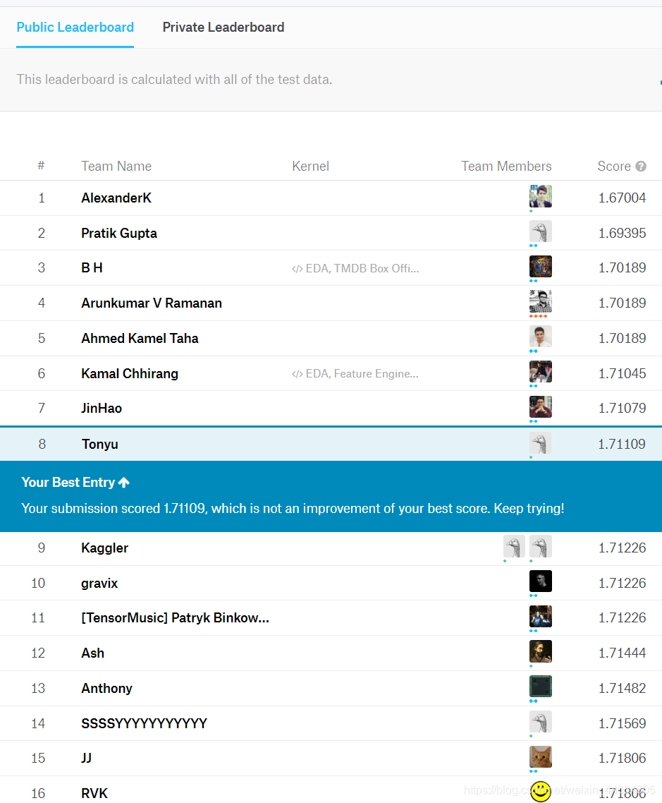
提交后就可以得到预测分数和名次了。
由于该比赛项目目前参赛人数不多,只有400只队伍,目前排名还比较靠前,是个不错的开始。接下来就可以尝试其他更多样的比赛了!