什么是回归分析
回归分析(regression analysis)是确定两种或两种以上变量间相互依赖的定量关系的一种统计分析方法。运用十分广泛,回归分析按照涉及的变量的多少,分为一元回归和多元回归分析;按照因变量的多少,可分为简单回归分析和多重回归分析;按照自变量和因变量之间的关系类型,可分为线性回归分析和非线性回归分析。如果在回归分析中,只包括一个自变量和一个因变量,且二者的关系可用一条直线近似表示,这种回归分析称为一元线性回归分析。如果回归分析中包括两个或两个以上的自变量,且自变量之间存在线性相关,则称为多重线性回归分析。
其实就是给你一些点,求线性方程
让直接入门吧
import numpy as np
import matplotlib.pyplot as plt
%matplotlib inline
x = np.linspace(0,30,50)
y = x+ 2*np.random.rand(50)
plt.figure(figsize=(10,8))
plt.scatter(x,

图上有50个点,赶紧来求线性方程吧
from sklearn.linear_model import LinearRegression  #导入线性回归
model = LinearRegression()  #初始化模型
x1 = x.reshape(-1,1)   # 将行变列  得到x坐标
y1 = y.reshape(-1,1)   # 将行变列  得到y坐标
model.fit(x1,y1)  #训练数据
model.predict(40) #预测下x=40 ,y的值
array([[40.90816511]]) # x=40的预测值
还是画个图来看看比较好
plt.figure(figsize=(12,8))
plt.scatter(x,y)
x_test = np.linspace(0,40).reshape(-1,1)
plt.plot(x_test,model.predict(x_test))

有图可我不知道方程的参数
都有model了怎么能不知道
model.coef_   #array([[1.00116024]])   斜率
model.intercept_   # array([0.86175551])  截距
y = 1.00116024 * x + 0.86175551
那怎么评价这个模型的好坏
当然是越靠近越好 不就是点到直线的距离的平方越小越好
np.sum(np.square(model.predict(x1) - y1))
16.63930773735106 # 这个不错,挺小的
我不信是最好的,那就稍稍加一点截距0.01
y2 = model.coef_*x1 + model.intercept_ + 0.01
np.sum(np.square(y2 - y1))   #  16.64430773735106
还是画个图
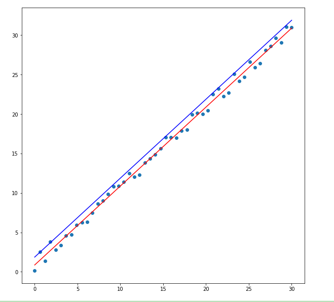
plt.figure(figsize=(10,10))
plt.scatter(x1,y1)
plt.plot(x1,model.predict(x1),color = 'r')
plt.plot(x1 , model.coef_*x1 + model.intercept_ +1, color = 'b')  # 用大的1区别这两条线,0.01两条线几乎重合