转载:火烫火烫的
个人觉得BP反向传播是深度学习的一个基础,所以很有必要把反向传播算法好好学一下
得益于一步一步弄懂反向传播的例子这篇文章,给出一个例子来说明反向传播
不过是英文的,如果你感觉不好阅读的话,优秀的国人已经把它翻译出来了。
一步一步弄懂反向传播的例子(中文翻译)
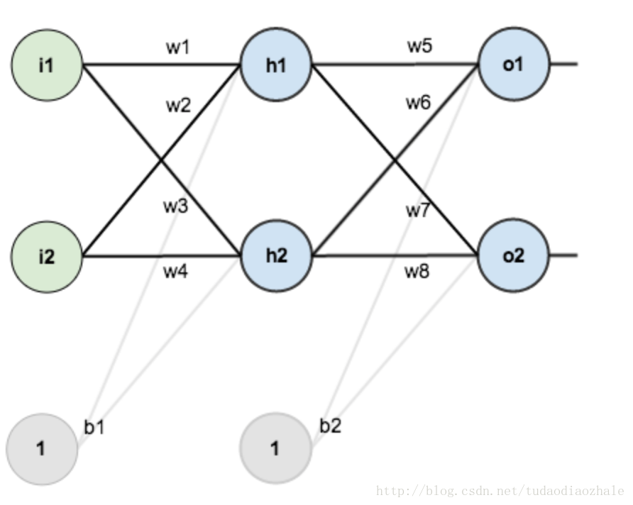
然后我使用了那个博客的图片。这次的目的主要是对那个博客的一个补充。但是首先我觉得先用面向过程的思想来实现一遍感觉会好一点。
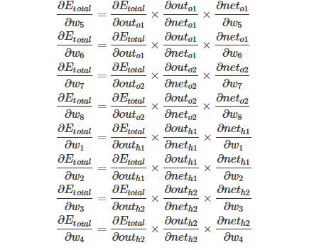
随便把文中省略的公式给大家给写出来。大家可以先看那篇博文
 1 import numpy as np
 2
 3 # "pd" 偏导
 4 def sigmoid(x):
 5     return 1 / (1 + np.exp(-x))
 6
 7 def sigmoidDerivationx(y):
 8     return y * (1 - y)
 9
10
11 if __name__ == "__main__":
12     #初始化
13     bias = [0.35, 0.60]
14     weight = [0.15, 0.2, 0.25, 0.3, 0.4, 0.45, 0.5, 0.55]
15     output_layer_weights = [0.4, 0.45, 0.5, 0.55]
16     i1 = 0.05
17     i2 = 0.10
18     target1 = 0.01
19     target2 = 0.99
20     alpha = 0.5 #学习速率
21     numIter = 10000 #迭代次数
22     for i in range(numIter):
23         #正向传播
24         neth1 = i1*weight[1-1] + i2*weight[2-1] + bias[0]
25         neth2 = i1*weight[3-1] + i2*weight[4-1] + bias[0]
26         outh1 = sigmoid(neth1)
27         outh2 = sigmoid(neth2)
28         neto1 = outh1*weight[5-1] + outh2*weight[6-1] + bias[1]
29         neto2 = outh2*weight[7-1] + outh2*weight[8-1] + bias[1]
30         outo1 = sigmoid(neto1)
31         outo2 = sigmoid(neto2)
32         print(str(i) + ", target1 : " + str(target1-outo1) + ", target2 : " + str(target2-outo2))
33         if i == numIter-1:
34             print("lastst result : " + str(outo1) + " " + str(outo2))
35         #反向传播
36         #计算w5-w8(输出层权重)的误差
37         pdEOuto1 = - (target1 - outo1)
38         pdOuto1Neto1 = sigmoidDerivationx(outo1)
39         pdNeto1W5 = outh1
40         pdEW5 = pdEOuto1 * pdOuto1Neto1 * pdNeto1W5
41         pdNeto1W6 = outh2
42         pdEW6 = pdEOuto1 * pdOuto1Neto1 * pdNeto1W6
43         pdEOuto2 = - (target2 - outo2)
44         pdOuto2Neto2 = sigmoidDerivationx(outo2)
45         pdNeto1W7 = outh1
46         pdEW7 = pdEOuto2 * pdOuto2Neto2 * pdNeto1W7
47         pdNeto1W8 = outh2
48         pdEW8 = pdEOuto2 * pdOuto2Neto2 * pdNeto1W8
49
50         # 计算w1-w4(输出层权重)的误差
51         pdEOuto1 = - (target1 - outo1) #之前算过
52         pdEOuto2 = - (target2 - outo2)  #之前算过
53         pdOuto1Neto1 = sigmoidDerivationx(outo1)    #之前算过
54         pdOuto2Neto2 = sigmoidDerivationx(outo2)    #之前算过
55         pdNeto1Outh1 = weight[5-1]
56         pdNeto2Outh2 = weight[7-1]
57
58         pdEOuth1 = pdEOuto1 * pdOuto1Neto1 * pdNeto1Outh1 + pdEOuto2 * pdOuto2Neto2 * pdNeto1Outh1
59         pdOuth1Neth1 = sigmoidDerivationx(outh1)
60         pdNeth1W1 = i1
61         pdNeth1W2 = i2
62         pdEW1 = pdEOuth1 * pdOuth1Neth1 * pdNeth1W1
63         pdEW2 = pdEOuth1 * pdOuth1Neth1 * pdNeth1W2
64         pdNeto1Outh2 = weight[6-1]
65         pdNeto2Outh2 = weight[8-1]
66         pdOuth2Neth2 = sigmoidDerivationx(outh2)
67         pdNeth2W3 = i1
68         pdNeth2W4 = i2
69         pdEOuth2 = pdEOuto1 * pdOuto1Neto1 * pdNeto1Outh2 + pdEOuto2 * pdOuto2Neto2 * pdNeto2Outh2
70         pdEW3 = pdEOuth2 * pdOuth2Neth2 * pdNeth2W3
71         pdEW4 = pdEOuth2 * pdOuth2Neth2 * pdNeth2W4
72         #权重更新
73         weight[1-1] = weight[1-1] - alpha * pdEW1
74         weight[2-1] = weight[2-1] - alpha * pdEW2
75         weight[3-1] = weight[3-1] - alpha * pdEW3
76         weight[4-1] = weight[4-1] - alpha * pdEW4
77         weight[5-1] = weight[5-1] - alpha * pdEW5
78         weight[6-1] = weight[6-1] - alpha * pdEW6
79         weight[7-1] = weight[7-1] - alpha * pdEW7
80         weight[8-1] = weight[8-1] - alpha * pdEW8
81         # print(weight[1-1])
82         # print(weight[2-1])
83         # print(weight[3-1])
84         # print(weight[4-1])
85         # print(weight[5-1])
86         # print(weight[6-1])
87         # print(weight[7-1])
88         # print(weight[8-1])
不知道你是否对此感到熟悉一点了呢?反正我按照公式实现一遍之后深有体会,然后用向量的又写了一次代码。
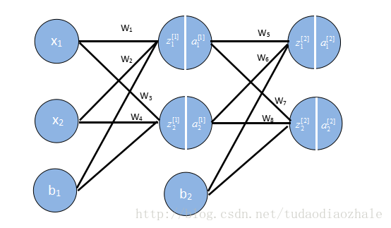
接下来我们要用向量来存储这些权重,输出结果等,因为如果我们不这样做,你看上面的例子就知道我们需要写很多w1,w2等,这要是参数一多就很可怕。
这些格式我是参考吴恩达的格式,相关课程资料->吴恩达深度学习视频。
 1 import numpy as np
 2
 3 def sigmoid(x):
 4     return 1 / (1 + np.exp(-x))
 5 def sigmoidDerivationx(y):
 6     return y * (1 - y)
 7
 8
 9 if __name__ == '__main__':
10     # 初始化一些参数
11     alpha = 0.5
12     numIter = 1000000 #迭代次数
13     w1 = [[0.15, 0.20], [0.25, 0.30]]  # Weight of input layer
14     w2 = [[0.40, 0.45], [0.50, 0.55]]
15     # print(np.array(w2).T)
16     b1 = 0.35
17     b2 = 0.60
18     x = [0.05, 0.10]
19     y = [0.01, 0.99]
20     # 前向传播
21     z1 = np.dot(w1, x) + b1     # dot函数是常规的矩阵相乘
22     a1 = sigmoid(z1)
23
24     z2 = np.dot(w2, a1) + b2
25     a2 = sigmoid(z2)
26     for n in range(numIter):
27         # 反向传播 使用代价函数为C=1 / (2n) * sum[(y-a2)^2]
28         # 分为两次
29         # 一次是最后一层对前面一层的错误
30
31         delta2 = np.multiply(-(y-a2), np.multiply(a2, 1-a2))
32         # for i in range(len(w2)):
33         #     print(w2[i] - alpha * delta2[i] * a1)
34         #计算非最后一层的错误
35         # print(delta2)
36         delta1 = np.multiply(np.dot(np.array(w2).T, delta2), np.multiply(a1, 1-a1))
37         # print(delta1)
38         # for i in range(len(w1)):
39             # print(w1[i] - alpha * delta1[i] * np.array(x))
40         #更新权重
41         for i in range(len(w2)):
42             w2[i] = w2[i] - alpha * delta2[i] * a1
43         for i in range(len(w1)):
44             w1[i] = w1[i] - alpha * delta1[i] * np.array(x)
45         #继续前向传播,算出误差值
46         z1 = np.dot(w1, x) + b1
47         a1 = sigmoid(z1)
48         z2 = np.dot(w2, a1) + b2
49         a2 = sigmoid(z2)
50         print(str(n) + " result:" + str(a2[0]) + ", result:" +str(a2[1]))
51         # print(str(n) + "  error1:" + str(y[0] - a2[0]) + ", error2:" +str(y[1] - a2[1]))
可以看到,用向量来表示的话代码就简短了非常多。但是用了向量化等的方法,如果不太熟,去看吴恩达深度学习的第一部分,再返过来看就能懂了。
扫描二维码关注公众号,回复:
101847 查看本文章
