论文学习：FCN（Fully Convolutional Networks for Semantic Segmentation）

论文原文：点击此处
论文下载：点击此处
论文被引：14541
论文年份：2014
论文代码：点击此处

顾名思义，fully convolutional networks 就是全卷积网络，那么它与传统的神经网络架构有什么区别？

• 没有全连接层，只有卷积层，有时还有池化层组成；
• 输入图像，输出也是图像，而不是分类，因为输出层是卷积层。
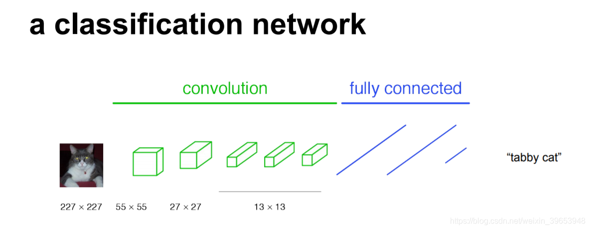
  看一下分类网络和FCN分割的对比。
  
  

这么做有什么优势？引用Quora上的一个回答1。

Input image size: If you don’t have any fully connected layer in your network, you can apply the network to images of virtually any size. Because only the fully connected layer expects inputs of a certain size, which is why in architectures like AlexNet, you must provide input images of a certain size (224x224).
Spatial information: Fully connected layer generally causes loss of spatial information - because its “fully connected”: all output neurons are connected to all input neurons. This kind of architecture can’t be used for segmentation, if you are working in a huge space of possibilities (e.g. unconstrained real images [1]). Although fully connected layers can still do segmentation if you are restricted to a relatively smaller space e.g. a handful of object categories with limited visual variation, such that the FC activations may act as a sufficient statistic for those images [2,3]. In the latter case, the FC activations are enough to encode both the object type and its spatial arrangement. Whether one or the other happens depends upon the capacity of the FC layer as well as the loss function.
Computational cost and representation power: There is also a distinction in terms of compute vs storage between convolutional layers and fully connected layers that I am a bit confused about. For instance, in AlexNet the convolutional layers comprised of 90% of the weights (~representational capacity) but contributed only to 10% of the computation; and the remaining (10% weights => less representation power, 90% computation) was eaten up by fully connected layers. Thus usually researchers are beginning to favor having a greater number of convolutional layers, tending towards fully convolutional networks for everything.

第二个回答2

Fully convolutional indicates that the neural network is composed of convolutional layers without any fully-connected layers or MLP usually found at the end of the network. A CNN with fully connected layers is just as end-to-end learnable as a fully convolutional one. The main difference is that the fully convolutional net is learning filters every where. Even the decision-making layers at the end of the network are filters.
A fully convolutional net tries to learn representations and make decisions based on local spatial input. Appending a fully connected layer enables the network to learn something using global information where the spatial arrangement of the input falls away and need not apply.

论文全文

全文较长，可以选择性阅读，论文全文为文字格式，Ctrl + F 检索定位。以前的文章只放了翻译校正后的中文，阅读起来反而有些属于不如英文清楚，于是翻译整理了英中对照，方便理解和阅读。

Fully Convolutional Networks for Semantic Segmentation

Abstract

Convolutional networks are powerful visual models that yield hierarchies of features. We show that convolutional networks by themselves, trained end-to-end, pixelstopixels, exceed the state-of-the-art in semantic segmentation.Our key insight is to build “fully convolutional” networks that take input of arbitrary size and produce correspondingly-sized output with efficient inference and learning. We define and detail the space of fully convolutional networks, explain their application to spatially dense prediction tasks, and draw connections to prior models. We adapt contemporary classification networks (AlexNet [22], the VGG net [34], and GoogLeNet [35]) into fully convolutional networks and transfer their learned representations by fine-tuning [5] to the segmentation task. We then define a skip architecture that combines semantic information from a deep, coarse layer with appearance information from a shallow, fine layer to produce accurate and detailed segmentations.Our fully convolutional network achieves stateofthe-art segmentation of PASCAL VOC (20% relative improvement to 62.2% mean IU on 2012), NYUDv2, and SIFT Flow, while inference takes less than one fifth of a second for a typical image.

卷积网络是强大的视觉模型，可产生要素层次结构。 我们证明，卷积网络本身（经过端到端训练的像素到像素）在语义分割方面超过了最新技术。我们的主要见识是建立“完全卷积”的网络，该网络可以接受任意大小的输入，并通过有效的推理和学习产生相应大小的输出。 我们定义和详细说明了全卷积网络的空间，解释了它们在空间密集的预测任务中的应用，并绘制了与先前模型的联系。 我们将当代分类网络（AlexNet [22]，VGG net [34]和GoogLeNet [35]）改编为完全卷积网络，并通过微调[5]将其学习的表示传递给分割任务。 然后，我们定义一个跳过体系结构，该体系结构将来自较深的粗糙层的语义信息与来自较浅的精细层的外观信息相结合，以产生准确而详细的细分。我们的完全卷积网络实现了PASCAL VOC（2012年相对改善，平均IU达到62.2％），NYUDv2和SIFT Flow的最新分割，而对于典型图像，推理所需的时间不到五分之一秒。

1. Introduction

卷积网络正在推动识别技术的进步。卷积不仅改善了全图像分类[22，34，35]，而且在具有结构化输出的本地任务上也取得了进展。 这些包括边界框对象检测[32、12、19]，部分和关键点预测[42、26]以及局部对应[26、10]方面的进步。

从粗略推断到精细推断的自然下一步是对每个像素进行预测。 先前的方法已经使用卷积语义分割[30、3、9、31、17、15、11]，其中每个像素都用其封闭的对象或区域的类别标记，但是存在该工作要解决的缺点。

我们显示，在语义分割上，经过端到端，像素到像素训练的完全卷积网络（FCN）超过了最新技术，而无需其他机制。据我们所知，这是端到端训练FCN的第一项工作（1）用于像素预测，而（2）则来自监督式预训练。 现有网络的完全卷积版本可以预测任意大小输入的密集输出。学习和推理都是通过密集的前馈计算和反向传播在整个图像时间进行的。网络内上采样层可通过子采样池在网络中实现像素级预测和学习。

这种方法在渐近性和绝对性上都是有效的，并且不需要其他工作中的复杂性。 逐块训练是常见的[30、3、9、31、11]，但缺乏完全卷积训练的效率。 我们的方法没有利用前后处理的复杂性，包括超像素[9，17]，建议[17，15]或通过随机字段或局部分类器进行的事后细化[9，17]。 我们的模型通过将分类网络重新解释为完全卷积并根据其学习表示进行微调，将最近在分类[22、34、35]中的成功转移到密集预测。 相反，以前的工作在没有监督预训练的情况下应用了小型卷积网络[9，31，30]。

语义分割面临着语义和位置之间的固有矛盾：全局信息解决了什么，而本地信息解决了什么。 深度特征层次结构在非线性1局部到全局金字塔中编码位置和语义。 我们定义了一个跳过体系结构，以利用此功能范围，该功能范围在4.2节中结合了深层，粗略，语义信息和浅层，精细，外观信息（参见图3）。

在下一部分中，我们将回顾有关深度分类网，FCN和使用卷积网络进行语义分割的最新方法的相关工作。 以下各节介绍了FCN设计和密集的预测权衡，介绍了具有网络内上采样和多层组合的体系结构，并描述了我们的实验框架。最后，我们演示了PASCAL VOC 2011-2，NYUDv2和SIFT Flow的最新结果。

2. Related work

我们的方法借鉴了深层网络在图像分类[22，34，35]和转移学习[5，41]方面的最新成功。 首先在各种视觉识别任务上演示了转移[5，41]，然后在混合提议分类器模型[12，17，15]中的检测以及实例和语义分割上进行了演示。 现在，我们重新架构和微调分类网，以进行语义细分的直接，密集的预测。 我们绘制了FCN的空间，并在此框架中建立了历史模型和最新模型。

完全卷积网络 据我们所知，将卷积网络扩展到任意大小的输入的想法首先出现在Matan等人中。 [28]扩展了经典的LeNet [23]以识别数字字符串。 因为它们的网络仅限于一维输入字符串，所以Matan等人。使用维特比解码获得其输出。 Wolf和Platt [40]将convnet输出扩展到邮政地址块四个角的检测分数的二维图。这两个历史著作都进行推理并完全卷积学习以进行检测。 宁等。 [30]定义了一个卷积网络，用于使用完全卷积推理对秀丽隐杆线虫组织进行粗分类。

在当今的多层网络时代，也已经开发了全卷积计算。 Sermanet等人的滑动窗口检测。 [32]，Pinheiro和Collobert [31]进行语义分割，以及Eigen等人进行图像复原。 [6]做全卷积推理。 完全卷积训练是很少见的，但是被汤普森等人有效地使用。 [38]学习一个端到端的零件检测器和空间模型来进行姿势估计，尽管它们没有阐述或分析这种方法。

另外，他等。 [19]丢弃分类网的非卷积部分以制作特征提取器。 他们将提案和空间金字塔池相结合，以产生用于分类的局部固定长度特征。 虽然快速有效，但无法端对端学习这种混合模型。

卷积网络的密集预测最近有几篇著作将卷积网络应用于密集的预测问题，包括Ning等人的语义分割。 [30]，Farabet等[9]，以及Pinheiro和Collobert [31]； Ciresan等人的电子显微镜边界预测。 [3]和Ganin和Lempitsky [11]的混合卷积/最近邻模型的自然图像； 以及Eigen等人的图像恢复和深度估计。 [6，7]。 这些方法的共同要素包括限制能力和接受范围的小模型；

• small models restricting capacity and receptive fields;
• patchwise training [30, 3, 9, 31, 11];
• post-processing by superpixel projection, random field regularization, filtering, or local classification [9, 3, 11];
• input shifting and output interlacing for dense output [32, 31, 11];
• multi-scale pyramid processing [9, 31, 11];
• saturating tanh nonlinearities [9, 6, 31]; and
• ensembles [3, 11],
  而我们的方法没有这种机制。 但是，我们确实从FCN的角度研究了分批训练3.4和“移位和缝合”密集输出3.2。 我们还将讨论网络中的上采样3.3，其中Eigen等人的预测是完全相关的。 [7]是一个特例。

与这些现有方法不同，我们采用图像分类作为监督的预训练来适应和扩展深度分类体系结构，并进行全面卷积微调，以从整个图像输入和整个图像地基中简单有效地学习。

Hariharan等。 [17]和古普塔等。 [15]同样使深度分类网适应语义分割，但在混合提议分类器模型中也是如此。 这些方法通过采样边界框和/或区域建议以进行检测，语义分割和实例分割来微调R-CNN系统[12]。 这两种方法都不是端到端学习的。 他们分别在PASCAL VOC和NYUDv2上实现了最新的分割结果，因此我们在第5节中直接将我们独立的端到端FCN与它们的语义分割结果进行比较。

我们跨层融合要素，以定义非线性的局部到全局表示，并进行端到端调整。 在当代作品中，Hariharan等人。 [18]在他们的混合模型中也使用了多层来进行语义分割。

3. Fully convolutional networks

Each layer of data in a convnet is a three-dimensional array of size h×w×d, where h and w are spatial dimensions, and d is the feature or channel dimension. The first layer is the image, with pixel size h×w, and d color channels.Locations in higher layers correspond to the locations in the image they are path-connected to, which are called their receptive fields.

卷积网络中的每一层数据都是尺寸为h×w×d的三维数组，其中h和w是空间维，而d是特征或通道维。 第一层是图像，像素大小为h×w，具有d个颜色通道。较高层中的位置对应于它们在路径上连接到的图像中的位置，称为它们的接收场。

Convnets are built on translation invariance. Their basic components (convolution, pooling, and activation functions) operate on local input regions, and depend only on relative spatial coordinates. Writing xij for the data vector at location (i; j) in a particular layer, and yij for the following layer, these functions compute outputs yij by
where k is called the kernel size, s is the stride or subsampling factor, and fks determines the layer type: a matrix multiplication for convolution or average pooling, a spatial max for max pooling, or an elementwise nonlinearity for an activation function, and so on for other types of layers.

卷积建立在翻译不变性上。 它们的基本组件（卷积，池化和激活函数）在局部输入区域上运行，并且仅取决于相对空间坐标。 将xij写入特定层中位置（i; j）的数据矢量，并将yij写入下一层，这些函数可通过以下方式计算输出yij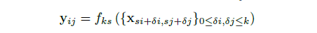
其中k称为内核大小，s为跨度或二次采样因子，fks确定层类型：用于卷积或平均池的矩阵乘法，用于最大池的空间最大值，或用于激活函数的元素非线性，等等 在其他类型的图层上。

This functional form is maintained under composition,with kernel size and stride obeying the transformation rule

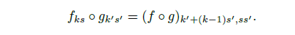
While a general deep net computes a general nonlinear function, a net with only layers of this form computes a nonlinear filter, which we call a deep filter or fully convolutional network. An FCN naturally operates on an input of any size, and produces an output of corresponding (possibly resampled) spatial dimensions.

该功能形式保持组成不变，内核大小和步幅遵循转换规则
一般的深层网络计算一般的非线性函数，而只有这种形式的层的网络计算非线性滤波器，我们称其为深层滤波器或完全卷积网络。 FCN自然可以在任何大小的输入上运行，并产生对应的（可能是重新采样的）空间尺寸的输出。
A real-valued loss function composed with an FCN defines a task. If the loss function is a sum over the spatial dimensions of the final layer,l(x; θ) = Σij ·l(xij ; θ), its gradient will be a sum over the gradients of each of its spatial components. Thus stochastic gradient descent on computed on whole images will be the same as stochastic gradient descent on l`, taking all of the final layer receptive fields as a minibatch.

由FCN组成的实值损失函数定义任务。 如果损失函数是最后一层空间维度上的总和，则l（x;θ）= ∑ij·l（xij;θ），其梯度将是其每个空间分量的梯度上的总和。 因此，将所有最终层接受场都作为一个小批量，对整个图像计算得出的上的随机梯度下降将与 l'上的随机梯度下降相同。

We next explain how to convert classification nets into fully convolutional nets that produce coarse output maps.For pixelwise prediction, we need to connect these coarse outputs back to the pixels. Section 3.2 describes a trick, fast scanning [13], introduced for this purpose. We gain insight into this trick by reinterpreting it as an equivalent network modification. As an efficient, effective alternative, we introduce deconvolution layers for upsampling in Section 3.3.In Section 3.4 we consider training by patchwise sampling, and give evidence in Section 4.3 that our whole image training is faster and equally effective.

接下来，我们将解释如何将分类网络转换为可生成粗糙输出图的全卷积网络。对于逐像素预测，我们需要将这些粗略输出连接回像素。 3.2节描述了一种技巧，即快速扫描[13]。 通过将其重新解释为等效的网络修改，我们可以深入了解此技巧。 作为一种有效的替代方法，我们将在第3.3节中介绍反卷积层以进行上采样。在第3.4节中，我们考虑通过逐点采样进行训练，并在第4.3节中提供证据，证明我们的整个图像训练更快且同样有效。

3.1. Adapting classifiers for dense prediction

Typical recognition nets, including LeNet [23], AlexNet [22], and its deeper successors [34, 35], ostensibly take fixed-sized inputs and produce non-spatial outputs. The fully connected layers of these nets have fixed dimensions and throw away spatial coordinates. However, these fully connected layers can also be viewed as convolutions with kernels that cover their entire input regions. Doing so casts them into fully convolutional networks that take input of any size and output classification maps. This transformation is illustrated in Figure 2.

典型的识别网络，包括LeNet [23]，AlexNet [22]及其更深的后继者[34、35]，表面上采用固定大小的输入并产生非空间输出。 这些网的完全连接的层具有固定的尺寸并丢弃空间坐标。 但是，这些完全连接的层也可以看作是覆盖整个输入区域的内核的卷积。 这样做会将它们投射到完全卷积的网络中，该网络可以接收任何大小的输入并输出分类图。 图2说明了这种转换。

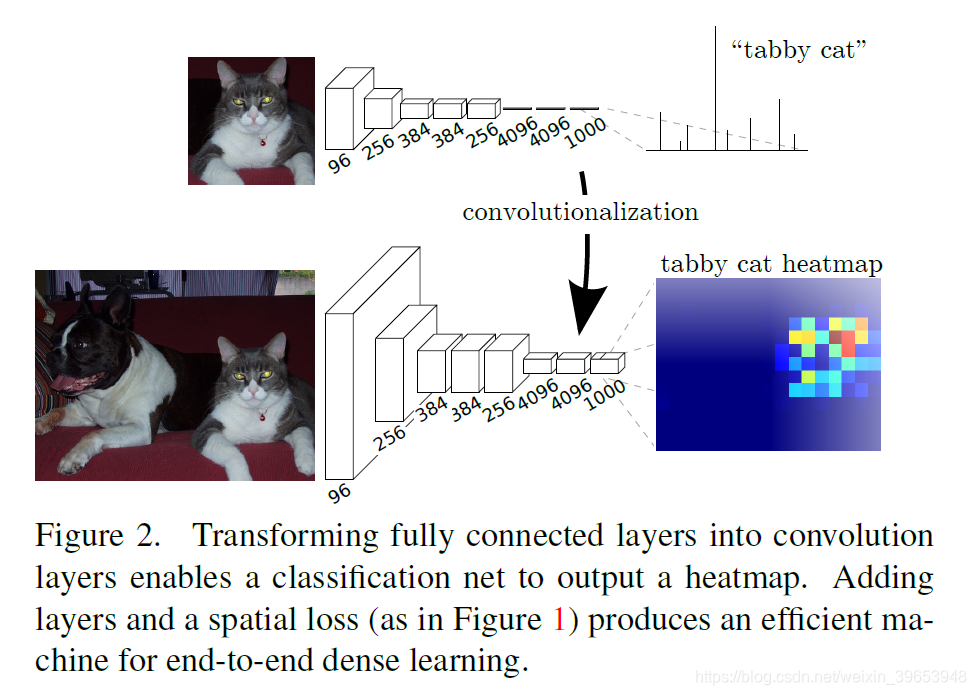
Furthermore, while the resulting maps are equivalent to the evaluation of the original net on particular input patches, the computation is highly amortized over the overlapping regions of those patches. For example, while AlexNet takes 1.2 ms (on a typical GPU) to infer the classification scores of a 227×227 image, the fully convolutional net takes 22 ms to produce a 10×10 grid of outputs from a 500×500 image, which is more than 5 times faster than the na¨ıve approach1.

此外，虽然生成的映射等效于在特定输入色块上对原始网络的评估，但在这些色块的重叠区域上进行了高额摊销。 例如，虽然AlexNet需要1.2毫秒（在典型的GPU上）来推断227×227图像的分类得分，但全卷积网络却需要22毫秒才能从500×500图像中生成10×10的输出网格。 比单纯的方法快5倍以上。

The spatial output maps of these convolutionalized models make them a natural choice for dense problems like semantic segmentation. With ground truth available at every output cell, both the forward and backward passes are straightforward, and both take advantage of the inherent computational efficiency (and aggressive optimization) of convolution. The corresponding backward times for the AlexNet example are 2.4 ms for a single image and 37 ms for a fully convolutional 10×10 output map, resulting in a speedup similar to that of the forward pass.

这些卷积模型的空间输出图使它们成为诸如语义分割之类的密集问题的自然选择。 由于每个输出单元都具有地面实况，向前和向后传递都很简单，并且都利用了卷积的固有计算效率（和主动优化）。 对于AlexNet示例，相应的后退时间对于单个图像是2.4毫秒，对于完全卷积的10×10输出映射是37毫秒，从而导致加速效果类似于正向传递。

While our reinterpretation of classification nets as fully convolutional yields output maps for inputs of any size, the output dimensions are typically reduced by subsampling.The classification nets subsample to keep filters small and computational requirements reasonable. This coarsens the output of a fully convolutional version of these nets, reducing it from the size of the input by a factor equal to the pixel stride of the receptive fields of the output units.

虽然我们将分类网重新解释为完全卷积的输出图，但对于任何大小的输入而言，输出尺寸通常都会通过子采样来降低。分类网子采样可保持过滤器较小且计算要求合理。 这使这些网络的完全卷积形式的输出变得粗糙，从而将其从输入大小中减小到等于输出单元接收场的像素跨度的倍数。

3.2. Shiftandstitch is filter rarefaction

Dense predictions can be obtained from coarse outputs by stitching together output from shifted versions of the input.If the output is downsampled by a factor of f, shift the input x pixels to the right and y pixels down, once for every (x; y) s.t. 0 ≤ x，y < f. Process each of these f² inputs, and interlace the outputs so that the predictions correspond to the pixels at the centers of their receptive fields.

通过将输入的移位版本的输出拼接在一起，可以从粗略的输出获得密集的预测。如果输出的下采样率为f，则将输入的x像素向右移动，将y像素向下移动，每·（x; y ）st 0≤x，y <f`。 处理这些 f ² 输入中的每个输入，并对输出进行隔行扫描，以使预测对应于其接收场中心的像素。

Although performing this transformation na¨ıvely increases the cost by a factor of f2, there is a well-known trick for efficiently producing identical results [13, 32] known to the wavelet community as the `a trous algorithm [27].Consider a layer (convolution or pooling) with input stride s, and a subsequent convolution layer with filter weights fij (eliding the irrelevant feature dimensions). Setting the lower layer’s input stride to 1 upsamples its output by a factor of s. However, convolving the original filter with the upsampled output does not produce the same result as shift-and-stitch, because the original filter only sees a reduced portion of its (now upsampled) input. To reproduce the trick, rarefy the filter by enlarging it as

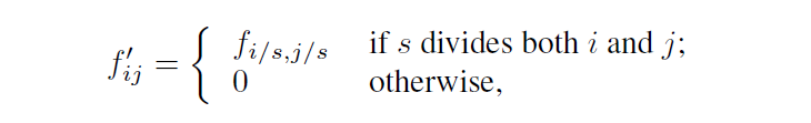
(with i and j zero-based). Reproducing the full net output of the trick involves repeating this filter enlargement layerby-layer until all subsampling is removed. (In practice, this can be done efficiently by processing subsampled versions of the upsampled input.)

尽管执行此转换会立即使成本增加f2倍，但有一个众所周知的技巧可以有效地产生相同的结果[13，32]，这对于小波社区来说是“ trous算法” [27]。考虑一个具有输入步幅s的层（卷积或池化），以及一个后续的卷积层，其滤波权重为fij（排除无关的特征尺寸）。 将较低层的输入步幅设置为1会将其输出上采样s倍。 但是，将原始滤波器与上采样输出进行卷积不会产生与移位和拼接相同的结果，因为原始滤波器只会看到其（现在是上采样）输入的减少部分。 要重现该技巧，请将过滤器放大为

（其中i和j从零开始）。 再现技巧的完整净输出涉及逐层重复此滤波器放大，直到删除所有子采样为止。 （实际上，这可以通过处理上采样输入的子采样版本来有效地完成。）
Decreasing subsampling within a net is a tradeoff: the filters see finer information, but have smaller receptive fields and take longer to compute. The shift-and-stitch trick is another kind of tradeoff: the output is denser without decreasing the receptive field sizes of the filters, but the filters are prohibited from accessing information at a finer scale than their original design.

减少网络内的二次采样是一个权衡：滤波器看到的信息更好，但接收场较小，计算所需的时间更长。 移位和缝合技巧是另一种折衷方案：输出更密集而不减小过滤器的接收场大小，但是与原始设计相比，过滤器被禁止以更精细的比例访问信息。

Although we have done preliminary experiments with this trick, we do not use it in our model. We find learning through upsampling, as described in the next section, to be more effective and efficient, especially when combined with the skip layer fusion described later on.

尽管我们已经使用此技巧进行了初步实验，但我们并未在模型中使用它。 我们发现，通过下采样进行学习（如下一节所述）更加有效，尤其是与稍后介绍的跳过层融合结合使用时。

3.3. Upsampling is backwards strided convolution

Another way to connect coarse outputs to dense pixels is interpolation. For instance, simple bilinear interpolation computes each output yij from the nearest four inputs by a linear map that depends only on the relative positions of the input and output cells.

将粗略输出连接到密集像素的另一种方法是插值。 例如，简单的双线性插值通过仅依赖于输入和输出像元的相对位置的线性映射从最近的四个输入计算每个输出 yij。

In a sense, upsampling with factor f is convolution with a fractional input stride of 1/f. So long as f is integral, a natural way to upsample is therefore backwards convolution (sometimes called deconvolution) with an output stride of f. Such an operation is trivial to implement, since it simply reverses the forward and backward passes of convolution.

从某种意义上说，因子为f的向上采样是卷积，输入步幅为1/f。 只要f是整数，向上采样的自然方法就是以输出步幅 f 向后进行卷积（有时称为反卷积）。 这样的操作很容易实现，因为它简单地反转了卷积的前进和后退。

Thus upsampling is performed in-network for end-to-end learning by backpropagation from the pixelwise loss.Note that the deconvolution filter in such a layer need not be fixed (e.g., to bilinear upsampling), but can be learned.A stack of deconvolution layers and activation functions can even learn a nonlinear upsampling.

因此，通过从像素方向的损失进行反向传播，在网络中执行上采样以进行端到端学习。注意，在这样的层中的去卷积滤波器不必是固定的（例如，固定为双线性上采样），而是可以学习的。一堆解卷积层和激活函数甚至可以学习非线性上采样。

In our experiments, we find that in-network upsampling is fast and effective for learning dense prediction. Our best segmentation architecture uses these layers to learn to upsample for refined prediction in Section 4.2.
在我们的实验中，我们发现网络内上采样对于学习密集预测是快速有效的。 我们最好的分割架构使用这些层来学习上采样，以进行第4.2节中的精确预测。

3.4. Patchwise training is loss sampling

In stochastic optimization, gradient computation is driven by the training distribution. Both patchwise training and fully convolutional training can be made to produce any distribution, although their relative computational efficiency depends on overlap and minibatch size. Whole image fully convolutional training is identical to patchwise training where each batch consists of all the receptive fields of the units below the loss for an image (or collection of images). While this is more efficient than uniform sampling of patches, it reduces the number of possible batches. However, random selection of patches within an image may be recovered simply. Restricting the loss to a randomly sampled subset of its spatial terms (or, equivalently applying a DropConnect mask [39] between the output and the loss) excludes patches from the gradient computation.

在随机优化中，梯度计算由训练分布驱动。 尽管它们的相对计算效率取决于重叠和最小批处理大小，但可以使补丁式训练和完全卷积训练两者都产生任何分布。 完整图像的全卷积训练与逐块训练相同，在该训练中，每批都包含低于图像损失（或图像收集）的单位的所有接受场。 虽然这比统一补丁采样更为有效，但它减少了可能的批次数量。 但是，可以简单地恢复图像内补丁的随机选择。 将损失限制为其空间项的随机采样子集（或等效地在输出和损失之间应用DropConnect掩码[39]）可将色块排除在梯度计算之外。

If the kept patches still have significant overlap, fully convolutional computation will still speed up training. If gradients are accumulated over multiple backward passes, batches can include patches from several images.²

如果保留的色块仍具有明显的重叠，则完全卷积计算仍将加快训练速度。 如果梯度是在多个向后遍历上累积的，则批处理可以包含来自多个图像的补丁。²

Sampling in patchwise training can correct class imbalance [30, 9, 3] and mitigate the spatial correlation of dense patches [31, 17]. In fully convolutional training, class balance can also be achieved by weighting the loss, and loss sampling can be used to address spatial correlation.

逐块训练中的采样可以纠正类不平衡[30、9、3]，并减轻密集块的空间相关性[31、17]。 在完全卷积训练中，也可以通过加权损失来实现类平衡，并且可以使用损失采样来解决空间相关性。

We explore training with sampling in Section 4.3, and do not find that it yields faster or better convergence for dense prediction. Whole image training is effective and efficient.

我们在第4.3节中探讨了采用采样的训练，但没有发现对于密集的预测它会产生更快或更佳的收敛。 整个图像训练是有效和高效的。

4. Segmentation Architecture

We cast ILSVRC classifiers into FCNs and augment them for dense prediction with in-network upsampling and a pixelwise loss. We train for segmentation by fine-tuning.Next, we add skips between layers to fuse coarse, semantic and local, appearance information. This skip architecture is learned end-to-end to refine the semantics and spatial precision of the output.

我们将ILSVRC分类器转换为FCN，并通过网络内上采样和逐像素损失对它们进行增强以进行密集的预测。 我们通过微调训练细分。接下来，我们在各层之间添加跳跃，以融合粗略的，语义的和局部的外观信息。 端到端学习了这种跳过架构，以改进输出的语义和空间精度。

For this investigation, we train and validate on the PASCAL VOC 2011 segmentation challenge [8]. We train with a per-pixel multinomial logistic loss and validate with the standard metric of mean pixel intersection over union, with the mean taken over all classes, including background. The training ignores pixels that are masked out (as ambiguous or difficult) in the ground truth.

对于此调查，我们训练并验证了PASCAL VOC 2011细分挑战[8]。 我们使用每像素多项式逻辑损失进行训练，并使用平均像素相交与并集的标准度量进行验证，并采用所有类别（包括背景）的均值。 训练会忽略在真实情况下被掩盖（模糊或困难）的像素。

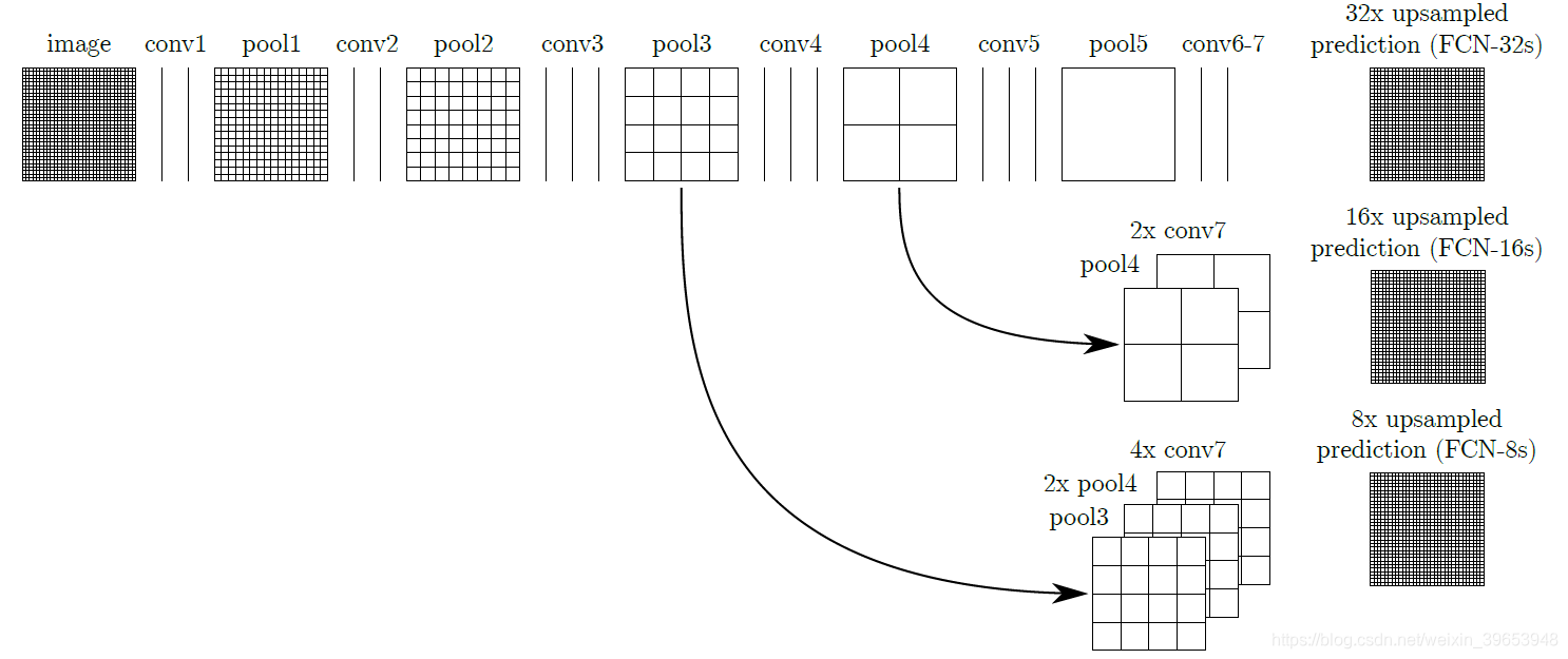
Figure 3. Our DAG nets learn to combine coarse, high layer information with fine, low layer information. Pooling and prediction layers are shown as grids that reveal relative spatial coarseness, while intermediate layers are shown as vertical lines. First row (FCN-32s): Our singlestream net, described in Section 4.1, upsamples stride 32 predictions back to pixels in a single step. Second row (FCN-16s): Combining predictions from both the final layer and the pool4 layer, at stride 16, lets our net predict finer details, while retaining high-level semantic information. Third row (FCN-8s): Additional predictions from pool3, at stride 8, provide further precision.

图3.我们的DAG网络学习将粗糙的高层信息与精细的低层信息相结合。 合并和预测层显示为显示相对空间粗糙度的网格，而中间层显示为垂直线。 第一行（FCN-32s）：如第4.1节所述，我们的单流网络将一步一步将32个预测返回到像素。 第二行（FCN-16）：在第16步结合来自最后一层和pool4层的预测，使我们的网络可以预测更精细的细节，同时保留高级语义信息。 第三行（FCN-8s）：在第8步中来自pool3的其他预测提供了更高的精度。

4.1. From classifier to dense FCN

We begin by convolutionalizing proven classification architectures as in Section 3. We consider the AlexNet³ architecture [22] that won ILSVRC12, as well as the VGG nets [34] and the GoogLeNet4 [35] which did exceptionally well in ILSVRC14. We pick the VGG 16-layer net5, which we found to be equivalent to the 19-layer net on this task. For GoogLeNet, we use only the final loss layer, and improve performance by discarding the final average pooling layer. We decapitate each net by discarding the final classifier layer, and convert all fully connected layers to convolutions. We append a 1×1 convolution with channel dimension 21 to predict scores for each of the PASCAL classes (including background) at each of the coarse output locations, followed by a deconvolution layer to bilinearly upsample the coarse outputs to pixel-dense outputs as described in Section 3.3. Table 1 compares the preliminary validation results along with the basic characteristics of each net. We report the best results achieved after convergence at a fixed learning rate (at least 175 epochs).

首先，如第3节所述，对经过验证的分类架构进行卷积。我们考虑赢得ILSVRC12的AlexNet³架构[22]，以及在ILSVRC14中表现出色的VGG网络[34]和GoogLeNet4 [35]。 我们选择了VGG 16层网络5，我们发现它相当于此任务上的19层网络。 对于GoogLeNet，我们仅使用最终的损失层，并通过丢弃最终的平均合并层来提高性能。 我们通过丢弃最终的分类器层来使每个网络断头，并将所有完全连接的层转换为卷积。 我们将通道尺寸为21的1×1卷积附加到每个粗略输出位置处的每个PASCAL类（包括背景）的分数预测中，然后进行解卷积层将粗略输出双线性升采样为像素密集输出，如所述 在第3.3节中。 表1比较了初步验证结果以及每个网络的基本特征。 我们报告了以固定的学习速度（至少175个epochs）收敛后获得的最佳结果。

Fine-tuning from classification to segmentation gave reasonable predictions for each net. Even the worst model achieved ~75% of state-of-the-art performance. The segmentation-equipped VGG net (FCN-VGG16) already appears to be state-of-the-art at 56.0 mean IU on val, compared to 52.6 on test [17]. Training on extra data raises FCN-VGG16 to 59.4 mean IU and FCN-AlexNet to 48.0 mean IU on a subset of val ⁷. Despite similar classification accuracy, our implementation of GoogLeNet did not match the VGG16 segmentation result.

从分类到细分的微调为每个网络提供了合理的预测。 即使是最差的型号，也可以达到约75％的最新性能。 配备分段功能的VGG网（FCN-VGG16）在val上的平均IU为56.0时已经是最新技术，而在测试时为52.6 [17]。 对额外数据的训练将val⁷的子集上的FCN-VGG16平均IU提高到59.4，将FCN-AlexNet的平均IU提高到48.0。 尽管分类精度相似，但我们的GoogLeNet实施与VGG16细分结果不匹配。

Table 1. We adapt and extend three classification convnets. We compare performance by mean intersection over union on the validation set of PASCAL VOC 2011 and by inference time (averaged over 20 trials for a 500×500 input on an NVIDIA Tesla K40c).We detail the architecture of the adapted nets with regard to dense prediction: number of parameter layers, receptive field size of output units, and the coarsest stride within the net. (These numbers give the best performance obtained at a fixed learning rate, not best performance possible.)

表1.我们适应并扩展了三个分类卷积。 我们通过PASCAL VOC 2011验证集上的平均交集与并集以及推理时间（在NVIDIA Tesla K40c上进行500×500输入的20多次试验平均）来比较性能。 预测：参数层数，输出单元的接收场大小以及网内最粗的步幅。 （这些数字给出了以固定学习率获得的最佳性能，而不是最佳性能。）

4.2. Combining what and where

We define a new fully convolutional net (FCN) for segmentation that combines layers of the feature hierarchy and refines the spatial precision of the output. See Figure 3.

我们定义了一种用于分割的新的全卷积网（FCN），该网结合了要素层次结构的各个层并完善了输出的空间精度。 参见图3。

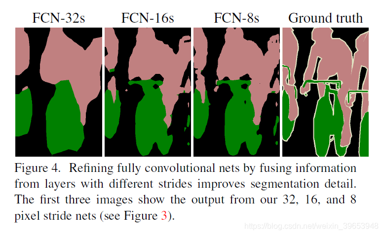
While fully convolutionalized classifiers can be finetuned to segmentation as shown in 4.1, and even score highly on the standard metric, their output is dissatisfyingly coarse (see Figure 4). The 32 pixel stride at the final prediction layer limits the scale of detail in the upsampled output.

尽管可以将完全卷积的分类器微调至如4.1所示的分段，甚至在标准度量上得分很高，但它们的输出却令人不满意地粗糙（请参见图4）。 最终预测层的32像素步幅限制了上采样输出中的细节比例。

We address this by adding skips [1] that combine the final prediction layer with lower layers with finer strides.This turns a line topology into a DAG, with edges that skip ahead from lower layers to higher ones (Figure 3). As they see fewer pixels, the finer scale predictions should need fewer layers, so it makes sense to make them from shallower net outputs. Combining fine layers and coarse layers lets the model make local predictions that respect global structure.By analogy to the jet of Koenderick and van Doorn [21], we call our nonlinear feature hierarchy the deep jet.

我们通过添加跳过[1]来解决此问题，这些跳过将最终预测层与较低层的步幅相结合。这会将线拓扑变成DAG，其边缘从较低的层向前跳到较高的层（图3）。 当他们看到较少的像素时，更精细的比例预测应该需要较少的图层，因此从较浅的净输出中进行选择是有意义的。 结合精细层和粗糙层，可以使模型做出尊重整体结构的局部预测。通过类似于Koenderick和van Doorn [21]的射流，我们将非线性特征层次称为深射流。

We first divide the output stride in half by predicting from a 16 pixel stride layer. We add a 1×1 convolution layer on top of pool4 to produce additional class predictions.We fuse this output with the predictions computed on top of conv7 (convolutionalized fc7) at stride 32 by adding a 2× upsampling layer and summing6 both predictions (see Figure 3). We initialize the 2× upsampling to bilinear interpolation, but allow the parameters to be learned as described in Section 3.3. Finally, the stride 16 predictions are upsampled back to the image. We call this net FCN-16s. FCN-16s is learned end-to-end, initialized with the parameters of the last, coarser net, which we now call FCN-32s. The new parameters acting on pool4 are zeroinitialized so that the net starts with unmodified predictions.The learning rate is decreased by a factor of 100.

我们首先根据16个像素的步幅层进行预测，将输出步幅分为两半。 我们在pool4的顶部添加一个1×1卷积层以产生附加的类别预测，并将此输出与在第32步的conv7（卷积化的fc7）顶部计算的预测相融合，方法是添加一个2×上采样层并对两个预测求和（请参见 图3）。 我们将2x上采样初始化为双线性插值，但允许按照第3.3节中的描述学习参数。 最后，将步幅16的预测上采样回图像。 我们称此为FCN-16s。 通过端到端学习FCN-16，并使用最后一个更粗糙的网络（现在称为FCN-32）的参数进行初始化。 作用于pool4的新参数被初始化为零，因此网络以未修改的预测开始。学习率降低了100倍。

Learning this skip net improves performance on the validation set by 3.0 mean IU to 62.4. Figure 4 shows improvement in the fine structure of the output. We compared this fusion with learning only from the pool4 layer, which resulted in poor performance, and simply decreasing the learning rate without adding the skip, which resulted in an insignificant performance improvement without improving the quality of the output.

学习此跳跃网可以将验证集的性能提高3.0个平均IU，达到62.4。 图4显示了输出精细结构的改进。 我们将这种融合与仅从pool4层进行的学习进行了比较，这导致性能较差，并且在不增加跳过的情况下简单地降低了学习速度，从而在不提高输出质量的情况下导致了微不足道的性能改进。

We continue in this fashion by fusing predictions from pool3 with a 2× upsampling of predictions fused from pool4 and conv7, building the net FCN-8s. We obtain a minor additional improvement to 62.7 mean IU, and find a slight improvement in the smoothness and detail of our output. At this point our fusion improvements have met diminishing returns, both with respect to the IU metric which emphasizes large-scale correctness, and also in terms of the improvement visible e.g. in Figure 4, so we do not continue fusing even lower layers.

我们以这种方式继续进行工作，将pool3的预测与pool4和conv7的预测进行2倍的上采样融合，构建净FCN-8。 我们将平均IU值略微提高了62.7 IU，并在输出的平滑度和细节上发现了轻微的改进。 在这一点上，我们的融合改进遇到了收益递减的问题，无论是在强调大规模正确性的IU度量方面，还是在可见的改进方面，例如 在图4中，因此我们不会继续融合更低的层。

Refinement by other means Decreasing the stride of pooling layers is the most straightforward way to obtain finer predictions. However, doing so is problematic for our VGG16-based net. Setting the pool5 stride to 1 requires our convolutionalized fc6 to have kernel size 14×14 to maintain its receptive field size. In addition to their computational cost, we had difficulty learning such large filters.We attempted to re-architect the layers above pool5 with smaller filters, but did not achieve comparable performance; one possible explanation is that the ILSVRC initialization of the upper layers is important.

通过其他手段进行优化减小池化层的步幅是获得更精细预测的最直接方法。 但是，这样做对于我们基于VGG16的网络是有问题的。 将pool5的跨度设置为1要求我们的卷积化的fc6具有14×14的内核大小，以维持其接收场大小。 除了计算量之外，我们还很难学习这么大的过滤器。我们试图用较小的过滤器重新构造pool5之上的层，但没有达到可比的性能； 一种可能的解释是高层的ILSVRC初始化很重要。

Another way to obtain finer predictions is to use the shiftandstitch trick described in Section 3.2. In limited experiments, we found the cost to improvement ratio from this method to be worse than layer fusion.

获得更好的预测的另一种方法是使用第3.2节中描述的shiftandstitch技巧。 在有限的实验中，我们发现此方法的成本改进率比层融合差。

4.3. Experimental framework

Optimization We train by SGD with momentum. We use a minibatch size of 20 images and fixed learning rates of 10^-3, 10^-4, and 5^-5 for FCN-AlexNet, FCN-VGG16, and FCN-GoogLeNet, respectively, chosen by line search. We use momentum 0:9, weight decay of 5^-4 or 2^-4, and doubled learning rate for biases, although we found training to be sensitive to the learning rate alone. We zero-initialize the class scoring layer, as random initialization yielded neither better performance nor faster convergence. Dropout was included where used in the original classifier nets.

优化我们通过SGD进行有动力的培训。 对于FCN-AlexNet，FCN-VGG16和FCN-GoogLeNet，我们分别使用20张图像的小批量大小和10 ^-3，10 ^-4和5 ^-5的固定学习率（按行选择） 搜索。 尽管我们发现训练仅对学习速率敏感，但我们使用动量为0：9，重量衰减为5 ^-4或2 ^-4，并将学习率提高了一倍。 我们将类计分层初始化为零，因为随机初始化既不会产生更好的性能，也不会带来更快的收敛。 在原始分类器网络中使用的地方包括了dropout。

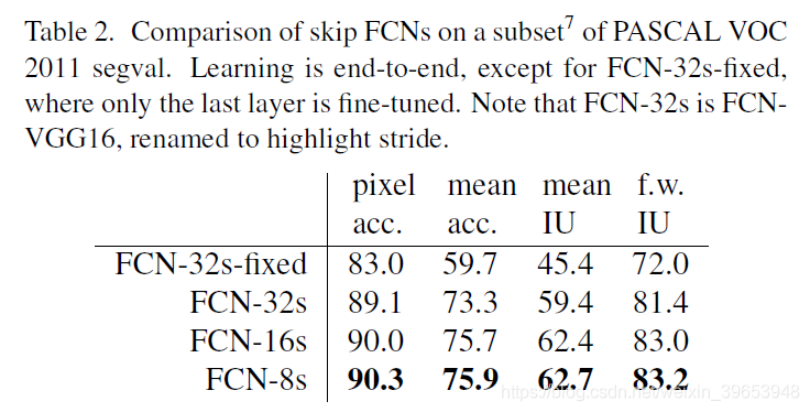
Fine-tuning We fine-tune all layers by backpropagation through the whole net. Fine-tuning the output classifier alone yields only 70% of the full finetuning performance as compared in Table 2. Training from scratch is not feasible considering the time required to learn the base classification nets. (Note that the VGG net is trained in stages, while we initialize from the full 16-layer version.) Fine-tuning takes three days on a single GPU for the coarse FCN-32s version, and about one day each to upgrade to the FCN-16s and FCN-8s versions.

微调我们通过整个网络的反向传播对所有层进行微调。 与表2相比，仅对输出分类器进行微调只能产生全部微调性能的70％。考虑到学习基础分类网络所需的时间，从头开始培训是不可行的。 （请注意，VGG网络是分阶段训练的，而我们是从完整的16层版本开始进行初始化的。）对于粗略的FCN-32s版本，微调在单个GPU上花费三天，而在每个GPU上升级大约需要一天。 FCN-16s和FCN-8s版本。

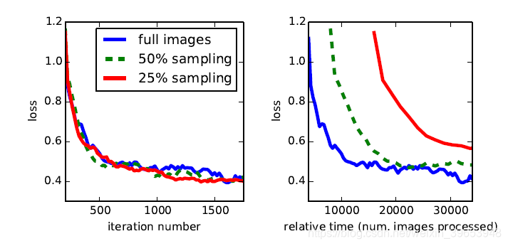
Figure 5. Training on whole images is just as effective as sampling patches, but results in faster (wall time) convergence by making more efficient use of data. Left shows the effect of sampling on convergence rate for a fixed expected batch size, while right plots the same by relative wall time.

图5.对整个图像进行训练与采样补丁一样有效，但是通过更有效地利用数据可以加快（墙时间）收敛。 左图显示了对于固定的预期批次大小，采样对收敛速度的影响，而右图则通过相对壁时间绘制了相同的结果。

More Training Data The PASCAL VOC 2011 segmentation training set labels 1112 images. Hariharan et al. [16] collected labels for a larger set of 8498 PASCAL training images, which was used to train the previous state-of-theart system, SDS [17]. This training data improves the FCNVGG16 validation score7 by 3.4 points to 59.4 mean IU.

更多培训数据PASCAL VOC 2011细分培训设置了1112张图像标签。 Hariharan等。 [16]收集了更大的8498 PASCAL训练图像集的标签，这些图像用于训练以前的最新系统SDS [17]。 该训练数据将FCNVGG16验证得分7提高了3.4点，至59.4平均IU。

Patch Sampling As explained in Section 3.4, our full image training effectively batches each image into a regular grid of large, overlapping patches. By contrast, prior work randomly samples patches over a full dataset [30, 3, 9, 31, 11], potentially resulting in higher variance batches that may accelerate convergence [24]. We study this tradeoff by spatially sampling the loss in the manner described earlier, making an independent choice to ignore each final layer cell with some probability 1-p. To avoid changing the effective batch size, we simultaneously increase the number of images per batch by a factor 1/p. Note that due to the efficiency of convolution, this form of rejection sampling is still faster than patchwise training for large enough values of p (e.g., at least for p > 0.2 according to the numbers in Section 3.1). Figure 5 shows the effect of this form of sampling on convergence. We find that sampling does not have a significant effect on convergence rate compared to whole image training, but takes significantly more time due to the larger number of images that need to be considered per batch. We therefore choose unsampled, whole image training in our other experiments.

补丁采样如第3.4节所述，我们的完整图像训练将每个图像有效地批量成大块重叠补丁的规则网格。 相比之下，先前的工作在整个数据集上随机采样补丁[30、3、9、31、11]，可能会导致更高的方差批次，从而可能加速收敛[24]。 我们通过以前面描述的方式对损失进行空间采样来研究这种折衷，并做出独立选择，以某些概率“ 1-p”忽略每个最终层单元。 为了避免更改有效的批次大小，我们同时将每批次的图像数量增加了“ 1 / p”。 注意，由于卷积的效率，对于足够大的“ p”值（例如，至少根据第3.1节中的“ p> 0.2”而言），这种形式的拒绝采样仍比分片训练更快。 图5显示了这种形式的抽样对收敛的影响。 我们发现，与整个图像训练相比，采​​样对收敛速度没有显着影响，但是由于每批需要考虑的图像数量更多，因此花费的时间明显更多。 因此，我们在其他实验中选择未采样的整体图像训练。

Class Balancing Fully convolutional training can balance classes by weighting or sampling the loss. Although our labels are mildly unbalanced (about 3/4 are background), we find class balancing unnecessary.

类平衡完全卷积训练可以通过加权或采样损失来平衡类。 尽管我们的标签略有不平衡（大约3 /4是背景），但我们发现类平衡是不必要的。

Dense Prediction The scores are upsampled to the input dimensions by deconvolution layers within the net. Final layer deconvolutional filters are fixed to bilinear interpolation, while intermediate upsampling layers are initialized to bilinear upsampling, and then learned.

密集预测通过网络中的反卷积层将分数上采样到输入维度。 最终层反卷积滤波器固定为双线性插值，而中间上采样层则初始化为双线性上采样，然后学习。

Augmentation We tried augmenting the training data by randomly mirroring and “jittering” the images by translating them up to 32 pixels (the coarsest scale of prediction) in each direction. This yielded no noticeable improvement.

增强我们尝试通过随机镜像和“抖动”图像​​来增强训练数据，方法是将图像在每个方向上最多转换为32个像素（最粗的预测比例）。 这没有产生明显的改善。

Implementation All models are trained and tested with Caffe [20] on a single NVIDIA Tesla K40c. Our models and code are publicly available at http://fcn.berkeleyvision.org.

实施所有模型都在单个NVIDIA Tesla K40c上使用Caffe [20]进行了培训和测试。 我们的模型和代码可在http://fcn.berkeleyvision.org上公开获得。

5. Results

We test our FCN on semantic segmentation and scene parsing, exploring PASCAL VOC, NYUDv2, and SIFT Flow. Although these tasks have historically distinguished between objects and regions, we treat both uniformly as pixel prediction. We evaluate our FCN skip architecture on each of these datasets, and then extend it to multi-modal input for NYUDv2 and multi-task prediction for the semantic and geometric labels of SIFT Flow.

我们在语义分割和场景解析方面测试了FCN，探索了PASCAL VOC，NYUDv2和SIFT Flow。 尽管这些任务历来在对象和区域之间有所区别，但我们将两者均视为像素预测。 我们在每个数据集上评估我们的FCN跳过体系结构，然后将其扩展到NYUDv2的多模式输入，以及SIFT Flow的语义和几何标签的多任务预测。

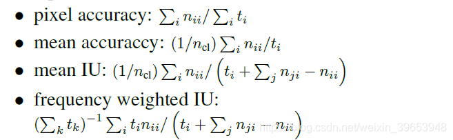
Metrics We report four metrics from common semantic segmentation and scene parsing evaluations that are variations on pixel accuracy and region intersection over union (IU). Let nij be the number of pixels of class i predicted to belong to class j, where there are ncl different classes, and letti = Σj·nijbe the total number of pixels of class i. We compute:

PASCAL VOC Table 3 gives the performance of our FCN-8s on the test sets of PASCAL VOC 2011 and 2012, and compares it to the previous state-of-the-art, SDS [17], and the well-known R-CNN [12]. We achieve the best results on mean IU⁸ by a relative margin of 20%. Inference time is reduced 114× (convnet only, ignoring proposals and refinement) or 286× (overall).

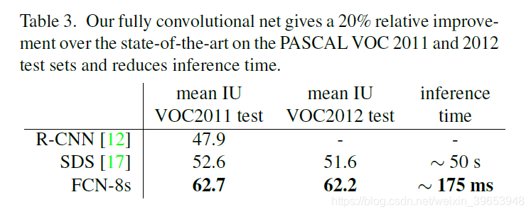
表4. NYUDv2上的结果。 RGBD是输入端的RGB和深度通道的早期融合。 HHA是[15]的深度嵌入，它是水平差异，离地面的高度以及局部表面法线与推断重力方向的角度。 RGB-HHA是联合训练的后期融合模型，将RGB和HHA预测相加。

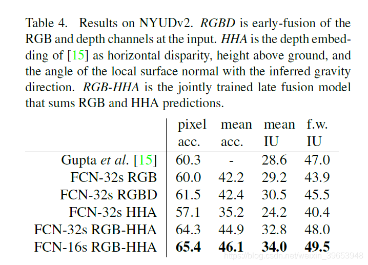
NYUDv2 [33] is an RGB-D dataset collected using the Microsoft Kinect. It has 1449 RGB-D images, with pixelwise labels that have been coalesced into a 40 class semantic segmentation task by Gupta et al. [14]. We report results on the standard split of 795 training images and 654 testing images. (Note: all model selection is performed on PASCAL 2011 val.) Table 4 gives the performance of our model in several variations. First we train our unmodified coarse model (FCN-32s) on RGB images. To add depth information, we train on a model upgraded to take four-channel RGB-D input (early fusion). This provides little benefit, perhaps due to the difficultly of propagating meaningful gradients all the way through the model. Following the success of Gupta et al. [15], we try the three-dimensional HHA encoding of depth, training nets on just this information, as well as a “late fusion” of RGB and HHA where the predictions from both nets are summed at the final layer, and the resulting two-stream net is learned end-to-end. Finally we upgrade this late fusion net to a 16-stride version.

NYUDv2 [33]是使用Microsoft Kinect收集的RGB-D数据集。 它具有1449个RGB-D图像，带有按像素划分的标签，由Gupta等人合并为40类语义分割任务。 [14]。 我们报告了795张训练图像和654张测试图像的标准分割结果。 （注意：所有模型的选择均在PASCAL 2011 val上进行。）表4给出了几种模型的性能。 首先，我们在RGB图像上训练未修改的粗糙模型（FCN-32s）。 为了增加深度信息，我们训练了一个升级后的模型，以采用四通道RGB-D输入（早期融合）。 这几乎没有好处，这可能是由于难以在模型中一直传播有意义的梯度。 继成功Gupta等。 [15]，我们尝试对深度进行三维HHA编码，仅在此信息上训练网络，以及RGB和HHA的“后期融合”，其中来自两个网络的预测在最后一层相加，并得出结果 两流网络是端到端学习的。 最后，我们将这个后期的融合网升级到16步的版本。

SIFT Flow is a dataset of 2,688 images with pixel labels for 33 semantic categories (“bridge”, “mountain”, “sun”), as well as three geometric categories (“horizontal”, “vertical”, and “sky”). An FCN can naturally learn a joint representation that simultaneously predicts both types of labels.
We learn a two-headed version of FCN-16s with semantic and geometric prediction layers and losses. The learned model performs as well on both tasks as two independently trained models, while learning and inference are essentially as fast as each independent model by itself. The results in Table 5, computed on the standard split into 2,488 training and 200 test images,9 show state-of-the-art performance on both tasks.

SIFT Flow是一个包含2688个图像的数据集，带有33个语义类别（“桥”，“山”，“太阳”）以及三个几何类别（“水平”，“垂直”和“天空”）的像素标签。 FCN可以自然地学习可以同时预测两种标签类型的联合表示。我们学习了带有语义和几何预测层以及损失的FCN-16的两头版本。 学习的模型在两个任务上的表现都好于两个独立训练的模型，而学习和推理在本质上与每个独立模型一样快。 表5中的结果按标准划分为2488个训练图像和200张测试图像9，显示出这两项任务的最新性能。

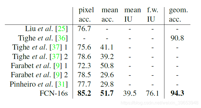
Table 5. Results on SIFT Flow⁹ with class segmentation (center) and geometric segmentation (right). Tighe [36] is a non-parametric transfer method. Tighe 1 is an exemplar SVM while 2 is SVM + MRF. Farabet is a multi-scale convnet trained on class-balanced samples (1) or natural frequency samples (2). Pinheiro is a multi-scale, recurrent convnet, denoted RCNN3 (o³). The metric for geometry is pixel accuracy.

表5. SIFT Flow ⁹ 的结果，包括类分割（中心）和几何分割（右）。 Tighe [36]是一种非参数传递方法。 Tighe 1是示例SVM，而2是SVM + MRF。 Farabet是在类平衡样本（1）或自然频率样本（2）上经过训练的多尺度卷积网络。 Pinheiro是一个多尺度的循环卷积网络，表示为RCNN3（o ³）。 几何指标是像素精度。

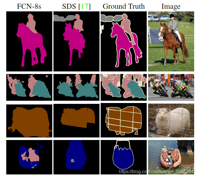
Figure 6. Fully convolutional segmentation nets produce stateofthe-art performance on PASCAL. The left column shows the output of our highest performing net, FCN-8s. The second shows the segmentations produced by the previous state-of-the-art system by Hariharan et al. [17]. Notice the fine structures recovered (first row), ability to separate closely interacting objects (second row), and robustness to occluders (third row). The fourth row shows a failure case: the net sees lifejackets in a boat as people.

图6.完全卷积分割网在PASCAL上表现出最先进的性能。 左列显示了性能最高的网络FCN-8的输出。 第二部分显示了Hariharan等人先前的最新系统所产生的分割结果。 [17]。 注意恢复的精细结构（第一行），分离紧密相互作用的对象的能力（第二行）以及对遮挡物的稳健性（第三行）。 第四行显示了一个失败案例：网络将船上的救生衣视为人。

6. Conclusion

Fully convolutional networks are a rich class of models, of which modern classification convnets are a special case. Recognizing this, extending these classification nets to segmentation, and improving the architecture with multi-resolution layer combinations dramatically improves the state-of-the-art, while simultaneously simplifying and speeding up learning and inference.

完全卷积网络是一类丰富的模型，现代分类卷积就是其中的特例。 认识到这一点，将这些分类网扩展到分段，并通过多分辨率图层组合改进体系结构，可以极大地改善现有技术，同时简化并加快学习和推理速度。

Acknowledgements This work was supported in part by DARPA’s MSEE and SMISC programs, NSF awards IIS1427425, IIS-1212798, IIS-1116411, and the NSF GRFP, Toyota, and the Berkeley Vision and Learning Center. We gratefully acknowledge NVIDIA for GPU donation. We thank Bharath Hariharan and Saurabh Gupta for their advice and dataset tools. We thank Sergio Guadarrama for reproducing GoogLeNet in Caffe. We thank Jitendra Malik for his helpful comments. Thanks to Wei Liu for pointing out an issue wth our SIFT Flow mean IU computation and an error in our frequency weighted mean IU formula.

A. Upper Bounds on IU

In this paper, we have achieved good performance on the mean IU segmentation metric even with coarse semantic prediction. To better understand this metric and the limits of this approach with respect to it, we compute approximate upper bounds on performance with prediction at various scales. We do this by downsampling ground truth images and then upsampling them again to simulate the best results obtainable with a particular downsampling factor. The following table gives the mean IU on a subset of PASCAL 2011 val for various downsampling factors.

在本文中，即使使用粗略的语义预测，我们在平均IU分割指标上也取得了良好的性能。 为了更好地理解该指标以及该方法相对于其的局限性，我们使用各种规模的预测来计算性能的近似上限。 为此，我们对地面真实图像进行下采样，然后再次对其进行上采样，以模拟使用特定下采样因子可获得的最佳结果。 下表列出了各种下采样因子下PASCAL 2011 val子集的平均IU。

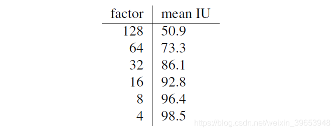
Pixel-perfect prediction is clearly not necessary to achieve mean IU well above state-of-the-art, and, conversely, mean IU is a not a good measure of fine-scale accuracy.

像素完美预测显然不需要达到远高于最新水平的平均IU，相反，平均IU并不是衡量小尺寸精度的好方法。

B. More Results

We further evaluate our FCN for semantic segmentation.
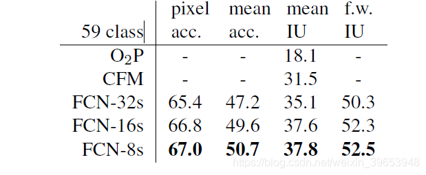
PASCAL-Context [29] provides whole scene annotations of PASCAL VOC 2010. While there are over 400 distinct classes, we follow the 59 class task defined by [29] that picks the most frequent classes. We train and evaluate on the training and val sets respectively. In Table 6, we compare to the joint object + stuff variation of Convolutional Feature Masking [4] which is the previous state-of-the-art on this task. FCN-8s scores 37.8 mean IU for a 20% relative improvement.

我们进一步评估FCN的语义分割。
PASCAL-Context [29]提供了PASCAL VOC 2010的整个场景注释。尽管有400多个不同的类，但我们遵循[29]定义的59类任务，该任务选择最频繁的类。 我们分别训练和评估训练集和评估集。 在表6中，我们将卷积特征蒙版[4]的联合对象+填充变量进行了比较，这是该任务的最新技术。 FCN-8s的平均IU得分为37.8，相对改善了20％。

Changelog

The arXiv version of this paper is kept up-to-date with corrections and additional relevant material. The following gives a brief history of changes.

本文的arXiv版本会进行更正和提供其他相关材料，以保持最新。 以下是更改的简要历史。

Table 6. Results on PASCAL-Context. CFM is the best result of [4] by convolutional feature masking and segment pursuit with the VGG net. O2P is the second order pooling method [2] as reported in the errata of [29]. The 59 class task selects the 59 most frequent classes for evaluation.

表6. PASCAL上下文的结果。 通过使用VGG网络进行卷积特征掩蔽和分段追踪，CFM是[4]的最佳结果。 O2P是[29]勘误中报告的第二级合并方法[2]。 59类任务选择59个最频繁的类进行评估。

v2 Add Appendix A giving upper bounds on mean IU and Appendix B with PASCAL-Context results. Correct PASCAL validation numbers (previously, some val images were included in train), SIFT Flow mean IU (which used an inappropriately strict metric), and an error in the frequency weighted mean IU formula. Add link to models and update timing numbers to reflect improved implementation (which is publicly available).

v2 添加附录A，以给出平均IU的上限，附录B为PASCAL-Context结果。 正确的PASCAL验证编号（以前在火车中包含一些val图像），SIFT流量平均IU（使用了不合适的严格度量）以及频率加权平均IU公式中的错误。 将链接添加到模型并更新时间编号以反映改进的实现（已公开）。

References

[1] C. M. Bishop. Pattern recognition and machine learning, page 229. Springer-Verlag New York, 2006. 6
[2] J. Carreira, R. Caseiro, J. Batista, and C. Sminchisescu. Semantic segmentation with second-order pooling. In ECCV, 2012. 9
[3] D. C. Ciresan, A. Giusti, L. M. Gambardella, and J. Schmidhuber.
Deep neural networks segment neuronal membranes in electron microscopy images. In NIPS, pages 2852–2860, 2012. 1, 2, 4, 7
[4] J. Dai, K. He, and J. Sun. Convolutional feature masking for joint object and stuff segmentation. arXiv preprint arXiv:1412.1283, 2014. 9
[5] J. Donahue, Y. Jia, O. Vinyals, J. Hoffman, N. Zhang, E. Tzeng, and T. Darrell. DeCAF: A deep convolutional activation feature for generic visual recognition. In ICML, 2014.
[6] D. Eigen, D. Krishnan, and R. Fergus. Restoring an image taken through a window covered with dirt or rain. In Computer Vision (ICCV), 2013 IEEE International Conference on, pages 633–640. IEEE, 2013. 2
[7] D. Eigen, C. Puhrsch, and R. Fergus. Depth map prediction from a single image using a multi-scale deep network. arXiv preprint arXiv:1406.2283, 2014. 2
[8] M. Everingham, L. Van Gool, C. K. I. Williams, J. Winn, and A. Zisserman. The PASCAL Visual Object Classes Challenge 2011 (VOC2011) Results. http://www.pascalnetwork.org/challenges/VOC/voc2011/workshop/index.html.
[9] C. Farabet, C. Couprie, L. Najman, and Y. LeCun. Learning hierarchical features for scene labeling. Pattern Analysis and Machine Intelligence, IEEE Transactions on, 2013. 1, 2, 4, 7, 8
[10] P. Fischer, A. Dosovitskiy, and T. Brox. Descriptor matching with convolutional neural networks: a comparison to SIFT.
CoRR, abs/1405.5769, 2014. 1
[11] Y. Ganin and V. Lempitsky. N4-fields: Neural network nearest neighbor fields for image transforms. In ACCV, 2014. 1, 2, 7
[12] R. Girshick, J. Donahue, T. Darrell, and J. Malik. Rich feature hierarchies for accurate object detection and semantic segmentation. In Computer Vision and Pattern Recognition, 2014. 1, 2, 7
[13] A. Giusti, D. C. Cires¸an, J. Masci, L. M. Gambardella, and J. Schmidhuber. Fast image scanning with deep max-pooling convolutional neural networks. In ICIP, 2013. 3, 4
[14] S. Gupta, P. Arbelaez, and J. Malik. Perceptual organization and recognition of indoor scenes from RGB-D images. In CVPR, 2013. 8
[15] S. Gupta, R. Girshick, P. Arbelaez, and J. Malik. Learning rich features from RGB-D images for object detection and segmentation. In ECCV. Springer, 2014. 1, 2, 8
[16] B. Hariharan, P. Arbelaez, L. Bourdev, S. Maji, and J. Malik.
Semantic contours from inverse detectors. In International Conference on Computer Vision (ICCV), 2011. 7
[17] B. Hariharan, P. Arbel´aez, R. Girshick, and J. Malik. Simultaneous detection and segmentation. In European Conference on Computer Vision (ECCV), 2014.
[18] B. Hariharan, P. Arbel´aez, R. Girshick, and J. Malik. Hypercolumns for object segmentation and fine-grained localization.
In Computer Vision and Pattern Recognition, 2015.
[19] K. He, X. Zhang, S. Ren, and J. Sun. Spatial pyramid pooling in deep convolutional networks for visual recognition. In ECCV, 2014.
[20] Y. Jia, E. Shelhamer, J. Donahue, S. Karayev, J. Long, R. Girshick, S. Guadarrama, and T. Darrell. Caffe: Convolutional architecture for fast feature embedding. arXiv preprint arXiv:1408.5093, 2014. 7
[21] J. J. Koenderink and A. J. van Doorn. Representation of local geometry in the visual system. Biological cybernetics, 55(6):367–375, 1987. 6
[22] A. Krizhevsky, I. Sutskever, and G. E. Hinton. Imagenet classification with deep convolutional neural networks. In NIPS, 2012. 1, 2, 3, 5
[23] Y. LeCun, B. Boser, J. Denker, D. Henderson, R. E. Howard, W. Hubbard, and L. D. Jackel. Backpropagation applied to hand-written zip code recognition. In Neural Computation, 1989. 2, 3
[24] Y. A. LeCun, L. Bottou, G. B. Orr, and K.-R. M¨uller. Efficient backprop. In Neural networks: Tricks of the trade, pages 9–48. Springer, 1998. 7
[25] C. Liu, J. Yuen, and A. Torralba. Sift flow: Dense correspondence across scenes and its applications. Pattern Analysis and Machine Intelligence, IEEE Transactions on, 33(5):978– 994, 2011. 8
[26] J. Long, N. Zhang, and T. Darrell. Do convnets learn correspondence?
In NIPS, 2014. 1
[27] S. Mallat. A wavelet tour of signal processing. Academic press, 2nd edition, 1999. 4
[28] O. Matan, C. J. Burges, Y. LeCun, and J. S. Denker. Multidigit recognition using a space displacement neural network.
In NIPS, pages 488–495. Citeseer, 1991. 2
[29] R. Mottaghi, X. Chen, X. Liu, N.-G. Cho, S.-W. Lee, S. Fidler, R. Urtasun, and A. Yuille. The role of context for object detection and semantic segmentation in the wild. In Computer Vision and Pattern Recognition (CVPR), 2014 IEEE Conference on, pages 891–898. IEEE, 2014. 9
[30] F. Ning, D. Delhomme, Y. LeCun, F. Piano, L. Bottou, and P. E. Barbano. Toward automatic phenotyping of developing embryos from videos. Image Processing, IEEE Transactions on, 14(9):1360–1371, 2005.[31] P. H. Pinheiro and R. Collobert. Recurrent convolutional neural networks for scene labeling. In ICML, 2014.
[32] P. Sermanet, D. Eigen, X. Zhang, M. Mathieu, R. Fergus, and Y. LeCun. Overfeat: Integrated recognition, localization and detection using convolutional networks. In ICLR, 2014.
[33] N. Silberman, D. Hoiem, P. Kohli, and R. Fergus. Indoor segmentation and support inference from rgbd images. In ECCV, 2012. 8
[34] K. Simonyan and A. Zisserman. Very deep convolutional networks for large-scale image recognition. CoRR, abs/1409.1556, 2014.
[35] C. Szegedy, W. Liu, Y. Jia, P. Sermanet, S. Reed, D. Anguelov, D. Erhan, V. Vanhoucke, and A. Rabinovich.
Going deeper with convolutions. CoRR, abs/1409.4842, 2014.
[36] J. Tighe and S. Lazebnik. Superparsing: scalable nonparametric image parsing with superpixels. In ECCV, pages 352– 365. Springer, 2010.
[37] J. Tighe and S. Lazebnik. Finding things: Image parsing with regions and per-exemplar detectors. In CVPR, 2013.
[38] J. Tompson, A. Jain, Y. LeCun, and C. Bregler. Joint training of a convolutional network and a graphical model for human pose estimation. CoRR, abs/1406.2984, 2014.
[39] L. Wan, M. Zeiler, S. Zhang, Y. L. Cun, and R. Fergus. Regularization of neural networks using dropconnect. In Proceedings of the 30th International Conference on Machine Learning (ICML-13), pages 1058–1066, 2013.
[40] R. Wolf and J. C. Platt. Postal address block location using a convolutional locator network. Advances in Neural Information Processing Systems, pages 745–745, 1994.
[41] M. D. Zeiler and R. Fergus. Visualizing and understanding convolutional networks. In Computer Vision–ECCV 2014, pages 818–833. Springer, 2014.
[42] N. Zhang, J. Donahue, R. Girshick, and T. Darrell. Partbased r-cnns for fine-grained category detection. In Computer Vision–ECCV 2014, pages 834–849. Springer, 2014.