1、图像轮廓和直方图
1.1 原理
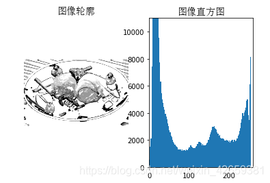
图像轮廓:绘制轮廓需要对每个坐标的像素值施加一个阈值,故首先将图像灰度化。
直方图:用来表征该图像像素值的分布情况。用一定的小区间来指定表征像素值的范围,每个小区间会得到落入该小区间表示范围的像素数目。图像直方图的绘制可以使用 hist() 函数。
convert()函数: PIL中有九种不同模式:1,L,P,RGB,RGBA,CMYK,YCbCr,I,F,其中模式"L"为灰色图像。convert(‘L’)表示将原图像转换成灰色图像。
flatten()函数 因为hist() 只接受一维数组作为输入,所以在绘制图像直方图之前,必须先对图像进行压平处理。flatten() 方法将任意数组按照行优先准则转换成一维数组。
1.2 代码实现及结果
# -*- coding: utf-8 -*-
from PIL import Image
from pylab import *

# 添加中文字体支持
from matplotlib.font_manager import FontProperties
font = FontProperties(fname=r"c:\windows\fonts\SimSun.ttc", size=14)
im = array(Image.open('c:/1.jpg').convert('L'))  # 打开图像,并转成灰度图像

figure()
subplot(121)
gray()
contour(im, origin='image')
axis('equal')
axis('off')
title(u'图像轮廓', fontproperties=font)

subplot(122)
hist(im.flatten(), 128)
title(u'图像直方图', fontproperties=font)
plt.xlim([0,260])
plt.ylim([0,11000])

show()
运行结果:
2、直方图均衡化
2.1 原理
直方图均衡化是将原图像通过某种变换,得到一幅灰度直方图为均匀分布的新图像的方法。直方图均衡化方法的基本思想是对在图像中像素个数多的灰度级进行展宽,而对像素个数少的灰度级进行缩减。从而达到清晰图像的目的。图像的均衡化直方图的绘制可以使用histeq()函数。
2.2 代码实现及结果
代码实现:
%matplotlib inline
# -*- coding: utf-8 -*-
from PIL import Image
from pylab import *
from PCV.tools import imtools

# 添加中文字体支持
from matplotlib.font_manager import FontProperties
font = FontProperties(fname=r"c:\windows\fonts\SimSun.ttc", size=14)

im = array(Image.open('c:/1.jpg').convert('L'))  # 打开图像,并转成灰度图像
#im = array(Image.open('../data/AquaTermi_lowcontrast.JPG').convert('L'))
im2, cdf = imtools.histeq(im)

figure()
subplot(2, 2, 1)
axis('off')
gray()
title(u'原始图像', fontproperties=font)
imshow(im)

subplot(2, 2, 2)
axis('off')
title(u'直方图均衡化后的图像', fontproperties=font)
imshow(im2)

subplot(2, 2, 3)
axis('off')
title(u'原始直方图', fontproperties=font)
#hist(im.flatten(), 128, cumulative=True, normed=True)
hist(im.flatten(), 128, normed=True)

subplot(2, 2, 4)
axis('off')
title(u'均衡化后的直方图', fontproperties=font)
#hist(im2.flatten(), 128, cumulative=True, normed=True)
hist(im2.flatten(), 128, normed=True)

show()
运行结果:
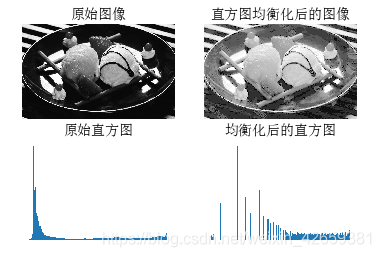
分析:
如上图所示,均衡化后的灰度图比原始图像的灰度图更亮、更清晰。经均衡化后的直方图分布比较均匀,而原始图像的直方图分布则相对没有那么均匀。
3、高斯滤波
3.1 原理
高斯滤波是一种线性平滑滤波,适用于消除高斯噪声,广泛应用于图像处理的减噪过程。高斯滤波就是对整幅图像进行加权平均的过程,每一个像素点的值,都由其本身和邻域内的其他像素值经过加权平均后得到。
高斯滤波的具体操作是:用一个模板(或称卷积、掩模)扫描图像中的每一个像素,用模板确定的邻域内像素的加权平均灰度值去替代模板中心像素点的值。
3.2 代码实现及结果
代码实现:
# -*- coding: utf-8 -*-
from PIL import Image
from pylab import *
from scipy.ndimage import filters

# 添加中文字体支持
from matplotlib.font_manager import FontProperties
font = FontProperties(fname=r"c:\windows\fonts\SimSun.ttc", size=14)

#im = array(Image.open('board.jpeg'))
im = array(Image.open('c:/1.jpg').convert('L'))

figure()
gray()
axis('off')
subplot(1, 4, 1)
axis('off')
title(u'原图', fontproperties=font)
imshow(im)

for bi, blur in enumerate([2, 5, 10]):
  im2 = zeros(im.shape)
  im2 = filters.gaussian_filter(im, blur)
  im2 = np.uint8(im2)
  imNum=str(blur)
  subplot(1, 4, 2 + bi)
  axis('off')
  title(u'标准差为'+imNum, fontproperties=font)
  imshow(im2)

#如果是彩色图像,则分别对三个通道进行模糊
#for bi, blur in enumerate([2, 5, 10]):
#  im2 = zeros(im.shape)
#  for i in range(3):
#    im2[:, :, i] = filters.gaussian_filter(im[:, :, i], blur)
#  im2 = np.uint8(im2)
#  subplot(1, 4,  2 + bi)
#  axis('off')
#  imshow(im2)

show()
运行结果:
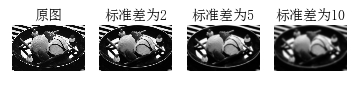
分析:
如上图所示,当高斯标准差分别为2、5、10时,高斯标准差为10的图像最模糊。即高斯标准差越大,图像越模糊。
