数字图像处理python基础 （一）

python图像处理基础（一）

写在前面的话： 方便以后查文档，且这篇文章会随着学习一直更（因为还有opencv还没怎么学，目前是一些基本的操作）。都是跟着学习资料巩固的，只供学习使用。

第一部分—— 图像基本操作

缩略图、截图、部分变换、旋转、图像转换为数组进行操作

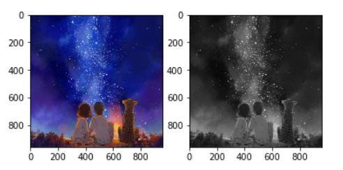
• 读取图片及灰度图

from PIL import Image #导入PIL库的Image类
import matplotlib.pyplot as plt

pil_im = Image.open('G:/photo/innovation/1.jpg') #读取图像文件
pil_im_gray = pil_im.convert('L')

plt.subplot(121)
plt.imshow(pil_im)
plt.subplot(122)
plt.imshow(pil_im_gray)

缩略图

thumbnail 或 resize

pil_im.thumbnail((128,128))
out= pil_im.resize((128,128))

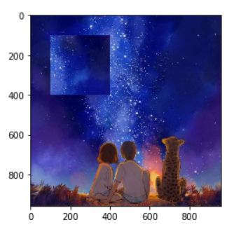
截图

（box is the crop rectangle, as a (left, upper, right, lower) tuple.）

box=(100,100,400,400)
region = pil_im.crop(box)

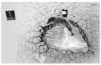
部分变换

transpose 之后 paste

region = region.transpose(Image.ROTATE_180)
pil_im.paste(region,box)

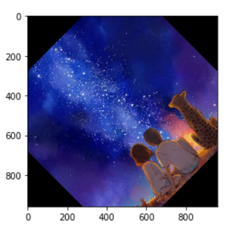
旋转

rotate() 传度数即可

out = pil_im.rotate(45)

图像转换为数组进行操作

可以对数组进行任意的灰度变换后再转换为图像输出

im = np.array(Image.open('G:/photo/innovation/1.jpg'))
print(im.shape, im.dtype)
pil_im = Image.fromarray(im)

第二部分—— 图像基本处理

灰度直方图、直方图均衡、空间滤波、图像基本变换、仿射变换

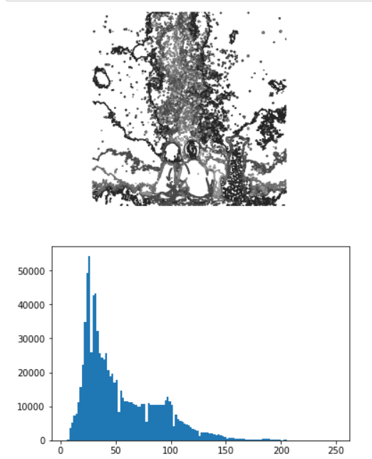
灰度直方图

contour作用是绘制等高线， hist 注意 im.flatten()

from PIL import Image
import numpy as np
import matplotlib.pyplot as plt
# read image to array
im = np.array(Image.open('G:/photo/innovation/1.jpg').convert('L'))
# create a new figure
plt.figure()
# don’t use colors
plt.gray()
# show contours with origin upper left corner
plt.contour(im, origin='image')
plt.axis('equal')
plt.axis('off')
plt.figure()
plt.hist(im.flatten(),128)
plt.show()

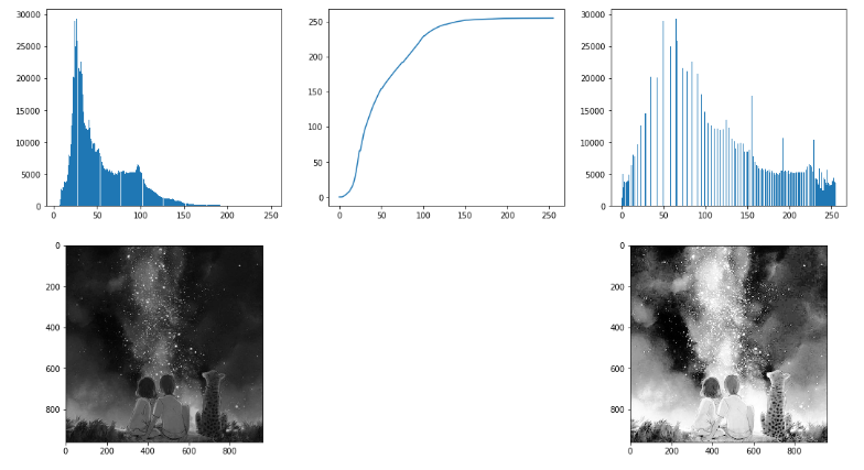
直方图均衡

$c(I) = \frac{1}{N} * \sum_{I=0}^{I}{h(i)} = c(I - 1) + \frac{1}{N} *h(I)$

我们要对图像求直方图，就需要先把图像矩阵进行flatten操作，使之变为一维数组，然后再进行统计用reshape进行变换，实际上变换后还是二维数组，两个方括号，因此只能用 flatten.

• cumsum(): 计算累计和
• flatten(): 个人理解为合并列表
• interp(): 线性插值函数
• numpy.interp(x, xp, fp, left=None, right=None, period=None)

def histeq(im,nbr_bins=256):
    """ Histogram equalization of a grayscale image. """

    # get image histogram
    imhist,bins = histogram(im.flatten(),nbr_bins,normed=True) 
    # 计算所有像素值
    cdf = imhist.cumsum() # cumulative distribution function 
    # 得出第一个乘数
    cdf = 255 * cdf / cdf[-1] # normalize
    
    # use linear interpolation of cdf to find new pixel values
    im2 = np.interp(im.flatten(),bins[:-1],cdf) 
    
    return im2.reshape(im.shape), cdf

from PIL import Image 
import numpy as np
im = array(Image.open('G:/photo/innovation/1.jpg').convert('L')) 
im2,cdf = histeq(im)

plt.figure(figsize=(18,10))
plt.subplot(231)
plt.hist(im.flatten(),256)
plt.subplot(232)
plt.plot(range(256),cdf)
plt.subplot(233)
plt.hist(im2.flatten(),256)
plt.subplot(234)
plt.gray()
plt.imshow(im)
plt.subplot(236)
plt.imshow(im2)

plt.show()

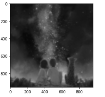
空间滤波

• 高斯滤波 gaussian_filter

from PIL import Image
import numpy as np
import matplotlib.pyplot as plt
from scipy.ndimage import filters

im = np.array(Image.open('G:/photo/innovation/1.jpg').convert('L')) 
im2 = filters.gaussian_filter(im,5)
pil_im2 = Image.fromarray(uint8(im2))
plt.imshow(pil_im2)

图像几何变换

SciPy库中的ndimage包的相关函数实现几何变换，ndimage.affine_transform

im = np.array(Image.open('G:/photo/innovation/1.jpg').convert('L'))
H = np.array([[1.4,0.05,-100],[0.05,1.5,-100],[0,0,1]])
im2 = ndimage.affine_transform(im,H[:2,:2],(H[0,2],H[1,2]))

plt.figure()
plt.gray()
plt.imshow(im2)
plt.show()

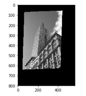
仿射变换

• 图像的坐标变换通常为仿射变换，其保留了共线性与距离比例
  • 共线性：变换前在同一直线上的点变换后还在同一直线上。
  • 距离比例：变换前后直线上各点之间的距离的比例保持不变。
• 仿射变换的一般形式

$u = c_{11}x + c_{12}y + c_{13}$ $v = c_{21}x + c_{22}y + c_{23}$

• $c_{13}, c_{23}$控制平移
• $c_{11}, c_{12}, c_{21}, c_{22}$控制缩放、旋转和剪切

接下来将一张图进行仿射变换后贴到另一张图的指定位置

def Haffine_from_points(fp,tp):
    """ Find H, affine transformation, such that tp is affine transf of fp. """
    
    if fp.shape != tp.shape:
        raise RuntimeError('number of points do not match')
    
    '''
    当 np.diag(array) 中,
    array是一个1维数组时，结果形成一个以一维数组为对角线元素的矩阵
    array是一个二维矩阵时，结果输出矩阵的对角线元素
    
    '''
    # condition points
    # --from points--
    m = np.mean(fp[:2], axis=1)
    maxstd = np.max(std(fp[:2], axis=1)) + 1e-9 
    C1 = np.diag([1/maxstd, 1/maxstd, 1]) 
    C1[0][2] = -m[0]/maxstd
    C1[1][2] = -m[1]/maxstd
    fp_cond = np.dot(C1,fp)
      
    # --to points--
    m = np.mean(tp[:2], axis=1)
    C2 = C1.copy() #must use same scaling for both point sets 
    C2[0][2] = -m[0]/maxstd
    C2[1][2] = -m[1]/maxstd
    tp_cond = np.dot(C2,tp)
    
    # conditioned points have mean zero, so translation is zero
    A = np.concatenate((fp_cond[:2],tp_cond[:2]), axis=0) 
    U,S,V = np.linalg.svd(A.T)

    # create B and C matrices as Hartley-Zisserman (2:nd ed) p 130.
    tmp = V[:2].T
    B = tmp[:2]
    C = tmp[2:4]
    
    '''
    vstack（）：堆栈数组垂直顺序（行）
    hstack（）：堆栈数组水平顺序（列）
    concatenate（）：连接沿现有轴的数组序列
    
    '''
    tmp2 = np.concatenate((dot(C,linalg.pinv(B)),zeros((2,1))), axis=1) 
    H = np.vstack((tmp2,[0,0,1]))
    # decondition
    H = dot(np.linalg.inv(C2),np.dot(H,C1)) 
    
    return H / H[2,2]

def image_in_image(im1,im2,tp):
    """ Put im1 in im2 with an affine transformation
    such that corners are as close to tp as possible.
    tp are homogeneous and counter-clockwise from top left. """
	
    # points to warp from
    m,n = im1.shape[:2]
    fp = np.array([[0,m,m,0],[0,0,n,n],[1,1,1,1]])
    # compute affine transform and apply
    H = Haffine_from_points(tp,fp)

    im1_t = ndimage.affine_transform(im1,H[:2,:2], (H[0,2],H[1,2]),im2.shape[:2])
    alpha = (im1_t > 0)
    
    return (1-alpha)*im2 + alpha*im1_t

# example of affine warp of im1 onto im2
im1 = np.array(Image.open('G:/photo/innovation/1.jpg').convert('L'))
im2 = np.array(Image.open('G:/photo/innovation/3.jpg').convert('L'))

tp = array([[158,310,304,141],[76,98,253,218],[1,1,1,1]]) 
im3 = image_in_image(im1,im2,tp)
plt.figure()
plt.gray()
plt.imshow(im3)
plt.axis('equal')
plt.axis('off')
plt.show()