OPENCV图像处理基础

1.图像处理基础
2.图像基本操作与opencv代码实现
3.图像分割与代码实现
4.图像特征提取与代码实现

1.图像处理基础

1.1 数字图像

1.1.1 数字图像概念：

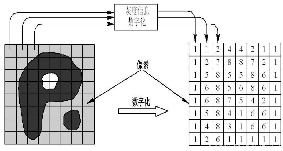
数字图像：又称数码图像，一幅二维图像可以由一个数组或矩阵表示。数字图像可以理解为一个二维函数f(x,y),其中x和y是空间（平面）坐标，而在任意坐标出的值f称为图像在该点处的强度或灰度。

图像处理的目的：改善图示的信息便于人们理解，有利于存储、传输和表示。
在这里插入图片描述

1.1.2 数字图像起源：

起源于20世纪20年代，媒体报纸业。

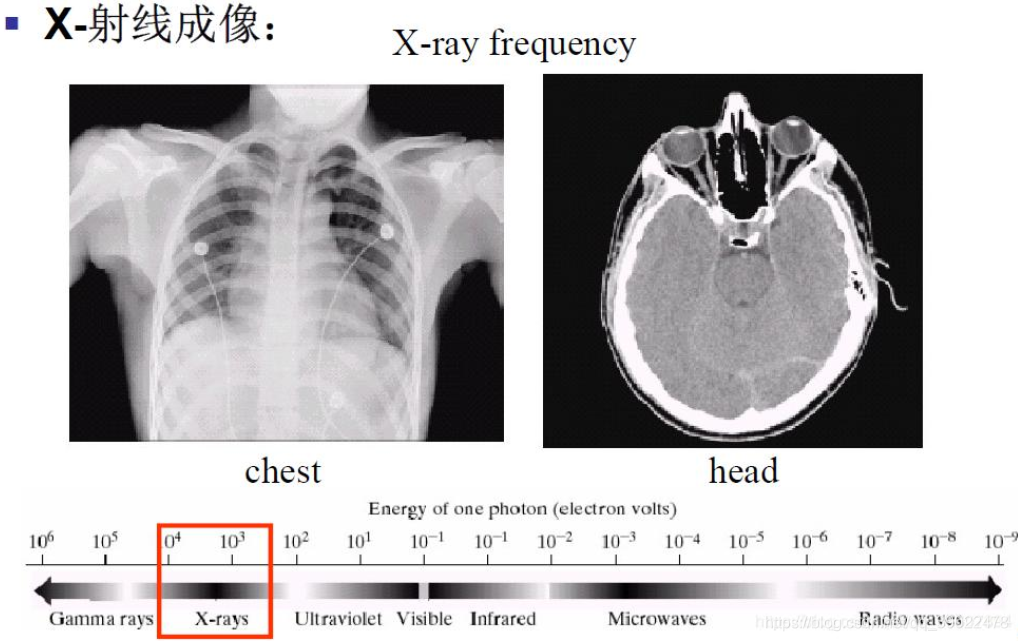
1.1.3 常见成像方式：

电磁波谱；γ射线成像；X射线成像；紫外线波段成像可见光波段成像；红外线波段成像等；
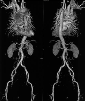
下图为X-射线成像：
在这里插入图片描述

1.1.4 数字图像的应用：

传统领域：医学，空间应用，生物学，军事
最新领域：数码相机，指纹识别，人脸识别，图像检索，游戏，电影特技等；
图像处理、机器视觉、人工智能关系：
图像处理主要研究二维图像，处理一个图像或一组图像之间的相互转换过程，包括图像滤波、图像识别、图像分割等；计算机视觉主要研究映射到单幅或多幅图像上的三维场景，从图像中提取抽象的语义信息，实现图像理解是计算机视觉的追求目标；人工智能在计算机视觉上的目标就是解决像素值和语义之间关系，主要的问题又图片检测、图片识别、图片分割和图片检索等。

1.1.5 Opencv介绍：

开源发行的跨平台计算机视觉库，是数字图像处理和计算机视觉领域非常常见的工具包
安装：打开终端/命令行cmd/虚拟环境，使用命令：pip install opencv-contrib-python 或 pip install opencv-python
如果安装失败，可先下载再使用pip命令安装，具体可参考相关教程。

1.2 图像属性

1.2.1 图像格式：

BMP格式：Windows系统下的标准位图格式，未经过压缩，一般图像文件比较大
JPEG格式：应用最广泛的格式之一，它采用一种特殊的有损压缩算法，达到较大的压缩比（可达到2：1甚至40：1）
GIF格式：可以是一张静止的图片，也可以是动画，支持透明背景图像，适用于多种操作系统，“体型”很小。但是其色域不太广，只支持256种颜色。
PNG格式：与JPG格式类似，压缩比高于GIF，支持图像透明，支持Alpha通道调节图像的透明度。
TIFF：特点是图像格式复杂，存储信息多，在Mac中广泛使用，非常有利于原稿的复制。很多地方将TIFF格式用于印刷。

注：JPEG和JPG区别可参考：https://www.zhihu.com/question/20329498。这里可理解为一个东西。

1.2.2 图像尺寸：

图像尺寸的长度和宽度以像素为单位。
像素（pixel）：像素是数码影像最基本的单位，每个像素就是一个小点，不同颜色的点聚集起来即成为一幅图片。灰度像素点数值范围在0到255之间，0表示黑，255表示白，其他值表示处于黑白之间；彩色图用红、绿、蓝三通道的二维矩阵来表示。每个数值也是在0~255之间，0表示相应的基色，而255则表示相应的基色在该像素中取得最大值。

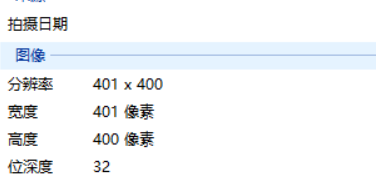
1.2.3 图像分辨率和通道：

分辨率：单位长度中的像素数目。每英寸图像中的像素点数，单位是像素每英寸（PPI）。图像分辨率越高，像素的点密度越高，图像越清晰。
通道数：图像的位深度，是指描述图像中每个pixel数值所占的二进制数。位深度越大则图像能表示的颜色数就越多，色彩越丰富逼真。

8位：单通道图像，也就是灰度图，灰度值范围2^8=256
24位：三通道3*8=24
32位：三通道加透明度Alpha通道

1.2.4 图像直方图：

图像直方图（Image Histogram）是用来表示数字图像中亮度分布的直方图，描绘了图像中每个亮度值的像素数。图像直方图中，横坐标左侧为纯黑、较暗的区域，右侧为较亮、纯白的区域。

图像直方图能表现出图像中的像素强度分布情况，它统计了每一个强度值所具有的像素个数。我们常借助图像直方图来实现图像的二值化。

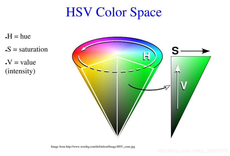
1.2.5 图像颜色空间：

概念：一种彩色模型，用途实在某些标准下用通常可接受的方式对彩色加以说明。
常见颜色空间：RGB HSV HSI CMYK

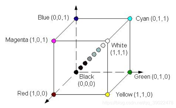
RGB颜色空间：依据人眼识别的颜色创建，图像中每一个像素都有R,G,B三个颜色分量组成，这三个大小均为【0，255】。通常表示某个颜色的时候，写成一个3维向量的形式，如（105，123，135）。
颜色模型：归一化后，原点（0，0，0)对应黑色，距原点最远的顶点对应白色，坐标为（1，1，1）；从黑色到白色的灰度值分布在这两个点的连线上，该虚线称为灰度线；立方体的其余各点对应不同的颜色，红绿蓝等等。
在这里插入图片描述
HSV颜色空间：根据颜色的直观特性创建的一种颜色空间。这个模型中颜色的参数分别是：色调（H），饱和度（S），明度（V）。
颜色模型：S通道，色彩/色调，代表颜色；S通道，饱和度，取值范围0%~100%，值越大颜色越饱和；V通道，明暗，数值越高越明亮，0%黑到100%白。
在这里插入图片描述

1.3 本章代码实现

1.读入图像
在这里插入图片描述

#导入opencv的python版本依赖库cv2
import cv2

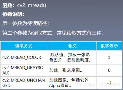
#使用opencv中imread函数读取图片，
#0代表灰度图形式打开，1代表彩色形式打开
img = cv2.imread('split.jpg',1)
print(img.shape)
#print(img)

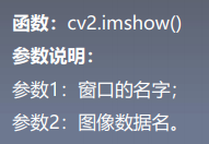
2.显示图像及保存图像（cv2和plt）
在这里插入图片描述

#导入opencv依赖库
import cv2

#读取图像，读取方式为彩色读取
img = cv2.imread('split.jpg',1)
#
cv2.imshow('photo',img)
k = cv2.waitKey(0)
if k == 27:   # 输入ESC键退出
    cv2.destroyAllWindows()
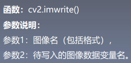
elif k == ord('s'): # 输入S键保存图片并退出
    cv2.imwrite('split_.jpg',img)
cv2.destroyAllWindows()

import cv2
from matplotlib import pyplot as plt

#使用Matplotlib导入图像
img = cv2.imread('test_image.png',0)
plt.imshow(img, cmap = 'gray', interpolation = 'bicubic')

#隐藏X、Y轴上的刻度
#plt.xticks([]), plt.yticks([])
plt.show()

3.通道转化，三通道转为单通道灰度图

在这里插入图片描述

import cv2 
#读入原始图像，使用cv2.IMREAD_UNCHANGED
img = cv2.imread("girl.jpg",cv2.IMREAD_UNCHANGED)
#查看打印图像的shape
shape = img.shape
print(shape)
#判断通道数是否为3通道或4通道
if shape[2] == 3 or shape[2] == 4 :
    #将彩色图转化为单通道图
    img_gray = cv2.cvtColor(img,cv2.COLOR_BGR2GRAY)
    cv2.imshow("gray_image",img_gray)
cv2.imshow("image", img)
cv2.waitKey(1000)
cv2.destroyAllWindows()

4.通道转化，单通道转为三通道灰度图

img_color = cv2.cvtColor(img,cv2.COLOR_GRAY2BGR)

5.图像通道分离与合并

import cv2 as cv
import numpy as np
src=cv.imread('split.jpg')
#cv.namedWindow('before',cv.WINDOW_NORMAL)
cv.imshow('before',src)
cv.waitKey(0)
#通道分离
b,g,r=cv.split(src)
cv.imshow('blue',b)
cv.imshow('green',g)
cv.imshow('red',r)
cv.waitKey(0)
#通道合并
#merge参数以list形式输入
src=cv.merge([b,g,r])
cv.imshow('merge',src)
cv.waitKey(0)
# 修改某个通道
src[:,:,2]=100
cv.imshow('single',src)
cv.waitKey(0)
cv.destroyAllWindows()

6.RGB转BGR

import cv2 
import matplotlib.pyplot as plt 
img = cv2.imread("test2.png", cv2.IMREAD_COLOR)
cv2.imshow("Opencv_win", img)
# 用opencv自带的方法转
img_cv_method = cv2.cvtColor(img, cv2.COLOR_BGR2RGB)
# 用numpy转，img[:,:,::-1]列左右翻转
img_numpy_method = img[:,:,::-1] # 本来是BGR 现在逆序，变成RGB
# 用matplot画图
plt.subplot(1,3,1)
plt.imshow(img_cv_method)
plt.subplot(1,3,2)
plt.imshow(img_numpy_method)
plt.subplot(1,3,3)
plt.imshow(img)
plt.savefig("./plt.png")
plt.show()
#保存图片
cv2.imwrite("opencv.png", img)
cv2.waitKey(0)
cv2.destroyAllWindows()

7.RGB与HSV转化

import cv2
#色彩空间转换函数
def color_space_demo(image):
    gray=cv2.cvtColor(image,cv2.COLOR_BGR2GRAY)
    cv2.imshow('gray',gray)
    hsv=cv2.cvtColor(image,cv2.COLOR_BGR2HSV)
    #print(hsv)
    cv2.imshow('hsv',hsv)
#读入一张彩色图
src=cv2.imread('girl.jpg')
cv2.imshow('before',src)
#调用color_space_demo函数进行色彩空间转化
color_space_demo(src)
cv2.waitKey(0)
cv2.destroyAllWindows()

8.绘制直方图
在这里插入图片描述

方法一

from matplotlib import pyplot as plt
import cv2

girl = cv2.imread("girl.jpg")
cv2.imshow("girl", girl)
# girl.ravel()函数是将图像的三位数组降到一维上去，
#256为bins的数目,[0, 256]为范围
plt.hist(girl.ravel(), 256, [0, 256])
plt.show()
cv2.waitKey(0)
cv2.destroyAllWindows()

方法二

from matplotlib import pyplot as plt
import cv2
import numpy as np
img = cv2.imread('girl.jpg')
img_gray = cv2.cvtColor(img, cv2.COLOR_BGR2GRAY)

plt.imshow(img_gray, cmap=plt.cm.gray)
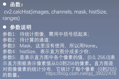
hist = cv2.calcHist([img], [0], None, [256], [0, 256])


plt.figure()
plt.title("Grayscale Histogram")
plt.xlabel("Bins")
plt.ylabel("# of Pixels")
plt.plot(hist)
plt.xlim([0, 256])
plt.show()

三通道直方图绘制

from matplotlib import pyplot as plt
import cv2
girl = cv2.imread("girl.jpg")
cv2.imshow("girl", girl)
color = ("b", "g", "r")
#使用for循环遍历color列表，enumerate枚举返回索引和值
for i, color in enumerate(color):
    hist = cv2.calcHist([girl], [i], None, [256], [0, 256])
    plt.title("girl")
    plt.xlabel("Bins")
    plt.ylabel("num of perlex")
    plt.plot(hist, color = color)
    plt.xlim([0, 260])
plt.show()
cv2.waitKey(0)
cv2.destroyAllWindows()

2.图像基本操作与opencv代码实现

2.1 Opencv中的绘图函数

1.线段绘制
在这里插入图片描述
2.矩形绘制

3.圆绘制

4.椭圆绘制

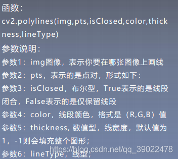
5.多边形绘制

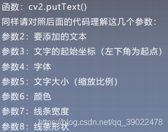
6.添加文字

7.代码实现

import numpy as np
import cv2

# 创建一张黑色的背景图
img=np.zeros((512,512,3), np.uint8)

# 绘制一条线宽为5的线段
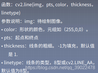
cv2.line(img,(0,0),(511,511),(255,0,0),1)

# 画一个绿色边框的矩形，参数2：左上角坐标，参数3：右下角坐标
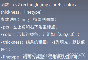
cv2.rectangle(img,(384,0),(510,128),(0,255,0),3)

# 画一个填充红色的圆，参数2：圆心坐标，参数3：半径
cv2.circle(img,(447,63), 63, (0,0,255), -1)

# 在图中心画一个填充的半圆
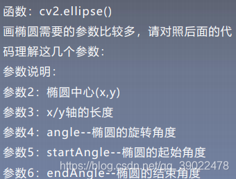
cv2.ellipse(img, (256, 256), (100, 50), 0, 0, 180, (255, 0, 0), -1)

#绘制多边形
pts=np.array([[10,5],[20,30],[70,20],[50,10]], np.int32)
pts=pts.reshape((-1,1,2))
cv2.polylines(img,[pts], True, (0,0,255),1)

# 这里 reshape 的第一个参数为-1, 表明这一维的长度是根据后面的维度的计算出来的。
#添加文字
font=cv2.FONT_HERSHEY_SIMPLEX
cv2.putText(img,'OpenCV',(10,500), font, 4,(255,255,255),2)


winname = 'example'
cv2.namedWindow(winname)
cv2.imshow(winname, img)
cv2.waitKey(0)
cv2.destroyWindow(winname)

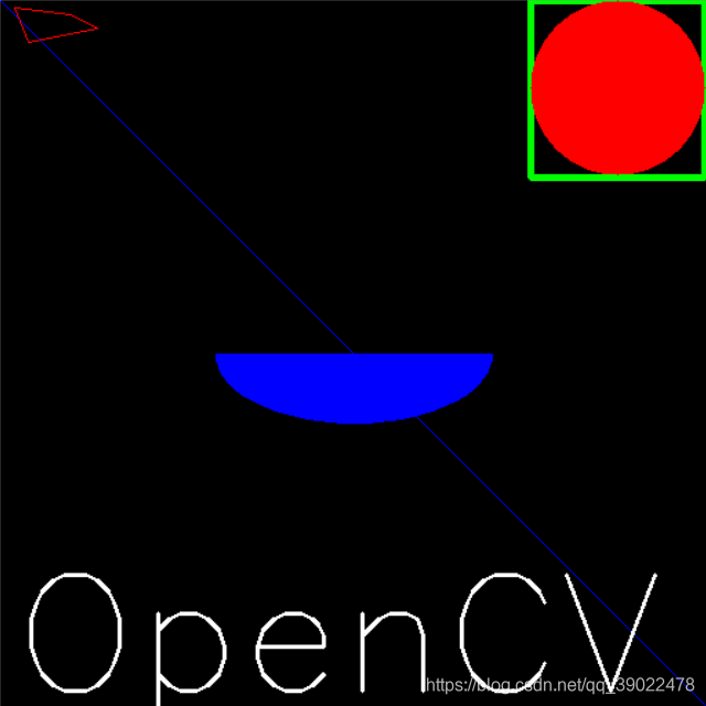
效果如下：
在这里插入图片描述

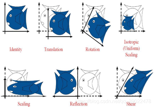
2.2 图像的几何变换

1.图像平移
将图像中所有的点按照指定的平移量水平或者垂直移动。
在这里插入图片描述

import cv2
import numpy as np
img = cv2.imread('img2.png')
# 构造移动矩阵H
# 在x轴方向移动多少距离，在y轴方向移动多少距离
H = np.float32([[1, 0, 50], [0, 1, 25]])
rows, cols = img.shape[:2]
print(img.shape)
print(rows, cols)

# 注意这里rows和cols需要反置，即先列后行
res = cv2.warpAffine(img, H, (2*cols, 2*rows))  
cv2.imshow('origin_picture', img)
cv2.imshow('new_picture', res)
cv2.waitKey(0)
cv2.destroyAllWindows()

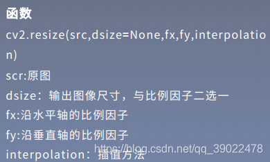
2.图像缩放
下采样：缩小图像称为下采样或降采样。
上采样：放大图像称为上采样。
图像缩放是指图像大小按照指定的比例或长宽进行放大或缩小。
在这里插入图片描述

import cv2
import numpy as np

img = cv2.imread('img2.png')
# 方法一：通过设置缩放比例，来对图像进行放大或缩小
res1 = cv2.resize(img, None, fx=2, fy=2, 
                  interpolation=cv2.INTER_CUBIC)
height, width = img.shape[:2]
# 方法二：直接设置图像的大小，不需要缩放因子
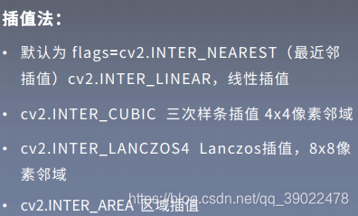
#cv2.INTER_NEAREST（最近邻插值） cv2.INTER_AREA （区域插值） cv2.INTER_CUBIC（三次样条插值） cv2.INTER_LANCZOS4（Lanczos插值）

res2 = cv2.resize(img, (int(0.8*width), int(0.8*height)),interpolation=cv2.INTER_LANCZOS4)
cv2.imshow('origin_picture', img)
#|cv2.imshow('res1', res1)
cv2.imshow('res2', res2)
cv2.waitKey(0)
cv2.destroyAllWindows()

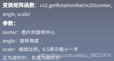
3.图像旋转
根据图像的旋转中心，将图像旋转一定的角度。旋转后图像的大小一般会改变，即可以把转出显示区域的图像截去，或者扩大图像范围来显示所有的图像。图像的旋转变换也可以用矩阵变换来表示。
设点p0(x,y)逆时针旋转θ角后的对应坐标为p(x,y),则p(x,y)为：
在这里插入图片描述
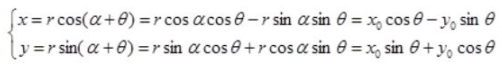
为避免信息的丢失，图像平移前应有一定的坐标平移。图像旋转后，会出现许多空洞点，对这些点需要进行填充处理。

import cv2
import numpy as np
img=cv2.imread('img2.png',1)
rows,cols=img.shape[:2]
#参数1：旋转中心，参数2：旋转角度，参数3：缩放因子
#参数3正为逆时针，负值为正时针
M=cv2.getRotationMatrix2D((cols/2,rows/2),45,1,)
print(M)
#第三个参数是输出图像的尺寸中心
dst=cv2.warpAffine(img,M,(cols,rows))
#borderValue为填充值
#dst=cv2.warpAffine(img,M,(cols,rows),borderValue=(255,255,255))
while(1):
    cv2.imshow('img', img)
    cv2.imshow('img1',dst)
    #0xFF==27  ESC
    if cv2.waitKey(1)&0xFF==27:
        break
cv2.destroyAllWindows()

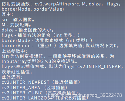
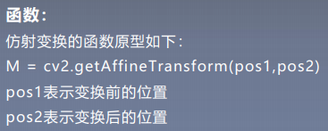
4.仿射变换
仿射变换是对图像进行旋转、平移、缩放等操作以达到数据增强的效果。
特点：变换前是直线，变换后依然是直线；直线的比例保持不变。
在这里插入图片描述

import cv2
import numpy as np
import matplotlib.pyplot as plt
#读取图片
src = cv2.imread('bird.png')
#获取图像大小
rows, cols = src.shape[:2]
#设置图像仿射变换矩阵
pos1 = np.float32([[50,50], [200,50], [50,200]])
pos2 = np.float32([[10,100], [200,50], [100,250]])
M = cv2.getAffineTransform(pos1, pos2)
print(M)
#图像仿射变换
result = cv2.warpAffine(src, M, (2*cols, 2*rows))
#显示图像
cv2.imshow("original", src)

cv2.imshow("result", result)
#等待显示
cv2.waitKey(0)
cv2.destroyAllWindows()

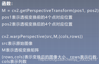
5.透视变化
将图像投影到一个新的视平面。
在这里插入图片描述

import cv2
import numpy as np
import matplotlib.pyplot as plt
#读取图片
src = cv2.imread('bird.png')
#获取图像大小
rows, cols = src.shape[:2]
#设置图像透视变换矩阵
pos1 = np.float32([[114, 82], [287, 156],
                   [8, 100], [143, 177]])
pos2 = np.float32([[0, 0], [188, 0], 
                   [0, 262], [188, 262]])
M = cv2.getPerspectiveTransform(pos1, pos2)
#图像透视变换
result = cv2.warpPerspective(src, M, (2*cols,2*rows))
#显示图像
cv2.imshow("original", src)
cv2.imshow("result", result)
#等待显示
cv2.waitKey(0)
cv2.destroyAllWindows()

6.文档矫正

#encoding:utf-8
import cv2
import numpy as np
import matplotlib.pyplot as plt

#读取图片
src = cv2.imread('paper.png')

#获取图像大小
rows, cols = src.shape[:2]

#将源图像高斯模糊
img = cv2.GaussianBlur(src, (3,3), 0)
#进行灰度化处理
gray = cv2.cvtColor(img,cv2.COLOR_BGR2GRAY)

#边缘检测（检测出图像的边缘信息）
edges = cv2.Canny(gray,50,250,apertureSize = 3)
cv2.imwrite("canny.jpg", edges)
cv2.imshow("canny", edges)
#通过霍夫变换得到A4纸边缘
lines = cv2.HoughLinesP(edges,1,np.pi/180,50,minLineLength=90,maxLineGap=10)
print(lines)
#下面输出的四个点分别为四个顶点
for x1,y1,x2,y2 in lines[0]:
    print(x1,y1)
    print(x2,y2)
for x3,y3,x4,y4 in lines[1]:
    print(x3,y3)
    print(x4,y4)

#绘制边缘
for x1,y1,x2,y2 in lines[0]:
    cv2.line(gray, (x1,y1), (x2,y2), (0,0,255), 1)

#根据四个顶点设置图像透视变换矩阵
pos1 = np.float32([[114, 82], [287, 156], [8, 322], [216, 333]]) 
pos2 = np.float32([[0, 0], [188, 0], [0, 262], [188, 262]])
M = cv2.getPerspectiveTransform(pos1, pos2)
# pos1 = np.float32([[114, 82], [287, 156], [8, 322]])
# pos2 = np.float32([[0, 0], [188, 0], [0, 262]])
# M = cv2.getAffineTransform(pos1,pos2)
print(M)
#图像仿射变换
#result = cv2.warpAffine(src, M, (2*cols, 2*rows))


#图像透视变换
result = cv2.warpPerspective(src, M, (190, 272))

#显示图像
cv2.imshow("original", src)
cv2.imshow("result", result)

cv2.imshow("gray", gray)
#等待显示
cv2.waitKey(0)
cv2.destroyAllWindows()

处理结果：
在这里插入图片描述

7.几何变换总结：

#encoding:utf-8
import cv2  
import numpy as np
import matplotlib.pyplot as plt
 
#读取图片
img = cv2.imread('test2.png')
image = cv2.cvtColor(img,cv2.COLOR_BGR2RGB)

#图像平移矩阵
M = np.float32([[1, 0, 80], [0, 1, 30]])
rows, cols = image.shape[:2]
img1 = cv2.warpAffine(image, M, (cols, rows))

#图像缩小
img2 = cv2.resize(image, (200,100))

#图像放大
img3 = cv2.resize(image, None, fx=1.1, fy=1.1)

#绕图像的中心旋转
#源图像的高、宽 以及通道数
rows, cols, channel = image.shape
#函数参数：旋转中心 旋转度数 scale
M = cv2.getRotationMatrix2D((cols/2, rows/2), 30, 1) 
#函数参数：原始图像 旋转参数 元素图像宽高
img4 = cv2.warpAffine(image, M, (cols, rows))

#图像翻转
img5 = cv2.flip(image, 0)   #参数=0以X轴为对称轴翻转 
img6 = cv2.flip(image, 1)   #参数>0以Y轴为对称轴翻转

#图像的仿射
pts1 = np.float32([[50,50],[200,50],[50,200]])
pts2 = np.float32([[10,100],[200,50],[100,250]])
M = cv2.getAffineTransform(pts1,pts2)
img7 = cv2.warpAffine(image, M, (rows,cols))

#图像的透射
pts1 = np.float32([[56,65],[238,52],[28,237],[239,240]])
pts2 = np.float32([[0,0],[200,0],[0,200],[200,200]])
M = cv2.getPerspectiveTransform(pts1,pts2)
img8 = cv2.warpPerspective(image,M,(200,200))


#循环显示图形
titles = [ 'source', 'shift', 'reduction', 'enlarge', 'rotation', 'flipX', 'flipY', 'affine', 'transmission']  
images = [image, img1, img2, img3, img4, img5, img6, img7, img8]  
for i in range(9):  
    plt.subplot(3, 3, i+1), plt.imshow(images[i], 'gray')  
    plt.title(titles[i])  
    plt.xticks([]),plt.yticks([])  
plt.show()

2.3 图像滤波与增强

滤波实际上是信号处理的一个概念，图像可以看成一个二维信号，其中像素点的灰度值代表信号的强弱。高频代表图像中变化剧烈的部分，低频代表灰度值变化平缓的区域。根据图像高低频，设计高通和低通滤波器。高通滤波器可以检测变化尖锐的地方，可用于边缘检测；低通滤波器可以让图像变得平滑，消除噪声，可用于平滑去噪。常见的线性滤波方式有方框滤波/均值滤波/公司滤波，非线性滤波有中值滤波/双边滤波。

图像滤波简介：
邻域算子：利用给定图像周围的像素值决定此像素的最终输出值的一种算子；
线性滤波：一种常用的邻域算子，像素输出取决于输入像素的加权和。
在这里插入图片描述
1.线性滤波：方框滤波
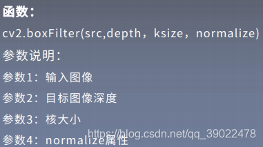
方框滤波（box Filter）被封装在boxFilter函数中，作用是使用方框滤波器来模糊一张图片，从src输入，从dst输出。
方框滤波核：

其中，α为：

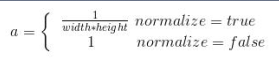
normalize=true时与均值滤波相同，normalize=false时易发生溢出。
在这里插入图片描述

import cv2
import numpy as np
img = cv2.imread('girl2.png',cv2.IMREAD_UNCHANGED)
r = cv2.boxFilter(img, -1 , (7,7) , normalize = 1)
d = cv2.boxFilter(img, -1 , (3,3) , normalize = 0)
cv2.namedWindow('img',cv2.WINDOW_AUTOSIZE)
cv2.namedWindow('r',cv2.WINDOW_AUTOSIZE)
cv2.namedWindow('d',cv2.WINDOW_AUTOSIZE)
cv2.imshow('img',img)
cv2.imshow('r',r)
cv2.imshow('d',d)
cv2.waitKey(0)
cv2.destroyAllWindows()

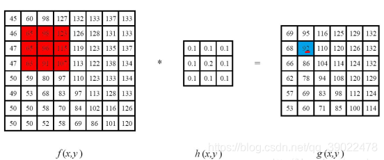
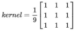
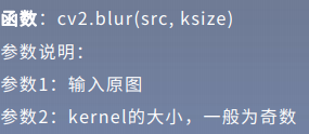
2.线性滤波：均值滤波
均值滤波是一种最简单的滤波处理，它取的是卷积核区域内元素的均值.如3*3的卷积核：
在这里插入图片描述

import cv2
import numpy as np
from matplotlib import pyplot as plt
img = cv2.imread('image/opencv.png')
cv2.imshow('img',img)
cv2.waitKey(0)
cv2.destroyAllWindows()
img = cv2.cvtColor(img,cv2.COLOR_BGR2RGB)
blur = cv2.blur(img,(3,3 ))
plt.subplot(121),plt.imshow(img),plt.title('Original')
plt.subplot(122),plt.imshow(blur),plt.title('Blurred')
plt.xticks([]), plt.yticks([])
plt.show()

3.线性滤波：高斯滤波
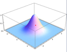
高斯滤波适用于消除高斯噪声，广泛应用于图像处理的减噪过程。高斯滤波的卷积核权重并不相同，中间像素点权重最高，越远离中心的像素权重越小。其原理是一个2维高斯函数。高斯滤波相比均值滤波效率较慢，但可以有效消除高斯噪声，能保留更多的图像细节。
在这里插入图片描述
opencv中的高斯滤波函数如下所示：

import cv2 as cv
import numpy as np
from matplotlib import pyplot as plt
img = cv.imread('image/median.png')
img = cv.cvtColor(img,cv.COLOR_BGR2RGB)
blur = cv.GaussianBlur(img,(7,7),7)
plt.subplot(121),plt.imshow(img),plt.title('Original')
plt.xticks([]), plt.yticks([])
plt.subplot(122),plt.imshow(blur),plt.title('Blurred')
plt.xticks([]), plt.yticks([])
plt.show()

4.非线性滤波：中值滤波
中值滤波是用像素点邻域灰度值的中值代替该点的灰度值，中值滤波可以去除椒盐噪声和斑点噪声。
在这里插入图片描述

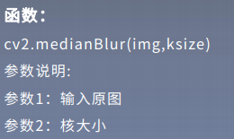
median = cv.medianBlur(img,3)

5.非线性滤波：双边滤波
双边滤波是结合图像的空间邻近度和像素值相似度的一种折中处理，同时考虑空间与信息和灰度相似性，达到保变去噪的目的，具有简单、非迭代、局部处理的特点。
在这里插入图片描述
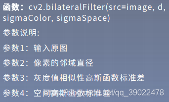
关于2个sigma参数：简单起见，可以令2个sigma的值相等；如果他们很小（小于10），那么滤波器几乎没有什么效果；如果他们很大（大于150），那么滤波器的效果会很强，使图像显得非常卡通化；
关于参数d：过大的滤波器（d>5）执行效率低。对于实时应用，建议取d=5；对于需要过滤严重噪声的离线应用，可取d=9； d>0时，由d指定邻域直径； d<=0时，d会自动由sigmaSpace的值确定，且d与sigmaSpace成正比；

import cv2
from matplotlib import pyplot as plt
img = cv2.imread('image/bilateral.png')
img = cv2.cvtColor(img,cv.COLOR_BGR2RGB)
blur = cv2.bilateralFilter(img,-1,15,10)
plt.subplot(121),plt.imshow(img),plt.title('Original')
plt.xticks([]), plt.yticks([])
plt.subplot(122),plt.imshow(blur),plt.title('Blurred')
plt.xticks([]), plt.yticks([])
plt.show()

**注：**opencv读取图像的方式是BGR,但是plt处理图像的方式是RGB，所以若想用plt显示图片需要先将BGR转为RGB。

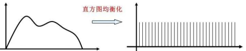
6.直方图均衡化
直方图均衡化是将原图像通过某种变换，得到一幅直方图为均匀分布的新图像的方法。
基本思想：对在图像中像素个数多的灰度级进行展宽，而对像素个数少的灰度级进行缩减。从而达到清晰图像的目的。
在这里插入图片描述

方法一：灰度图均衡化

import cv2
#直接读为灰度图像
img = cv2.imread('./image/dark.png',0)
cv2.imshow("dark",img)
cv2.waitKey(0)
#调用cv2.equalizeHist函数进行直方图均衡化
img_equal = cv2.equalizeHist(img)

cv2.imshow("img_equal",img_equal)
cv2.waitKey(0)
cv2.destroyAllWindows()

方法二：灰度图局部直方图均衡化

#调用cv2.createCLAHE函数进行局部直方图均衡化
clahe = cv2.createCLAHE(clipLimit=2,tileGridSize=(30,30))
cl1 = clahe.apply(img)

方法三：彩色图像均衡化

import cv2
import numpy as np
img = cv2.imread("./image/dark1.jpg")
cv2.imshow("src", img)
# 彩色图像均衡化,需要分解通道 对每一个通道均衡化
(b, g, r) = cv2.split(img)
bH = cv2.equalizeHist(b)
gH = cv2.equalizeHist(g)
rH = cv2.equalizeHist(r)
# 合并每一个通道
result = cv2.merge((bH, gH, rH))
cv2.imshow("dst", result)
cv2.waitKey(0)
cv2.destroyAllWindows()

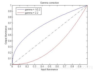
7.Gamma变换
Gamma变换是对图像灰度值进行的非线性操作，使输出图像灰度值与输入图像灰度值呈指数关系： $V_out = AV_in$
Gamma变换可以用来增强图像，其提升了暗部细节，通过非线性变换，让图像从曝光强度的线性响应变得更接近人眼感受的响应，即将漂白（相机曝光）或过暗（曝光不足）的图片进行矫正。
在这里插入图片描述

import cv2
import numpy as np
img=cv2.imread('./image/dark1.jpg')
def adjust_gamma(image, gamma=1.0):
    invGamma = 1.0/gamma
    table = []
    for i in range(256):
        table.append(((i / 255.0) ** invGamma) * 255)
    table = np.array(table).astype("uint8")
    print(table)
    return cv2.LUT(image, table)

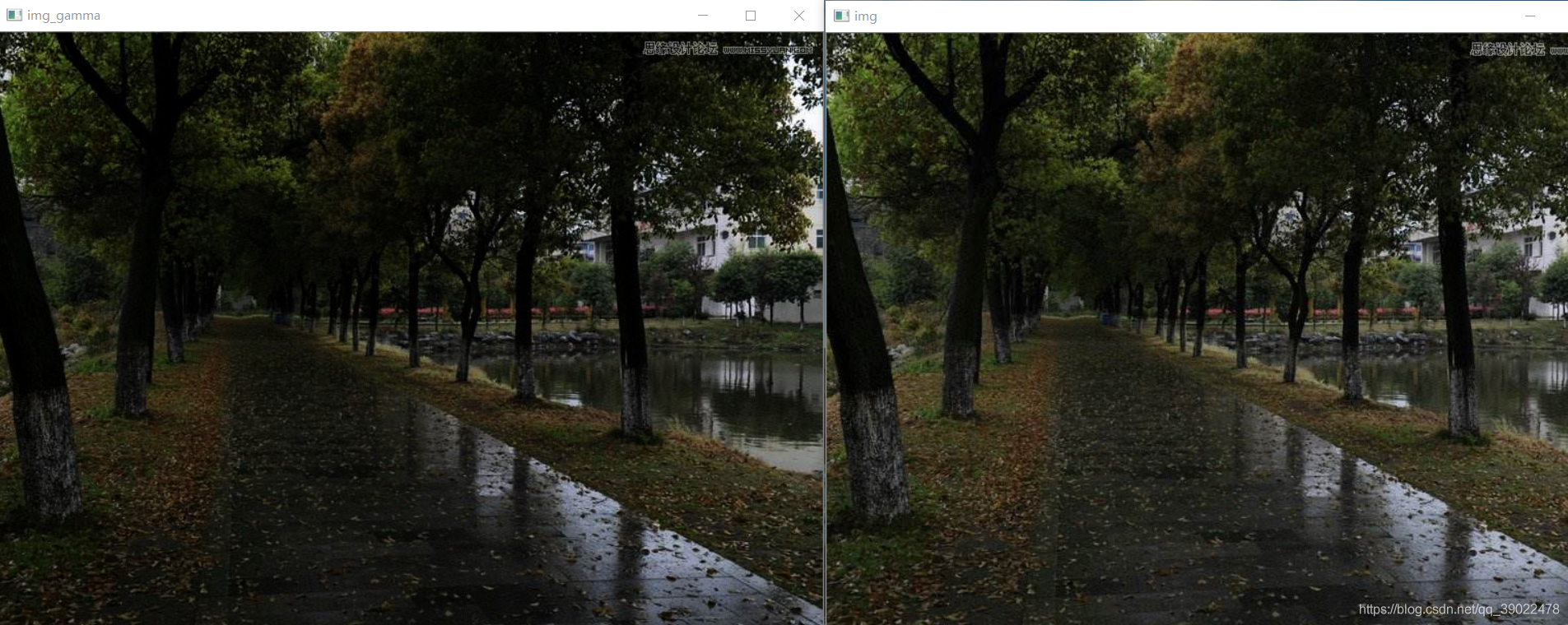
img_gamma = adjust_gamma(img, 0.8)
#print(img_gamma)
cv2.imshow("img",img)
cv2.imshow("img_gamma",img_gamma)

cv2.waitKey(0)
cv2.destroyAllWindows()

运行结果：
在这里插入图片描述

2.4 形态学操作

形态学，是图像处理中应用最为广泛的技术之一，主要用于从图像中提取对表达和描绘区域形状有意义的图像分量，使后续的识别工作能够抓住目标对象最为本质的形状特征，如边界和连通区域等。

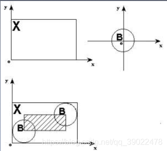
结构元素：设有两幅图像B,X。若X是被处理的对象，而B是用来处理X的，则称B为结构元素，又被称为刷子。结构元素通常是一些比较小的图像。

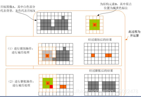
1.图像腐蚀
腐蚀类似于“领域被蚕食”，将图像中白色部分进行缩减细化，其运行结果图比原图的白色区域更小。

腐蚀的运算符是“ - ”，其定义如下：
在这里插入图片描述
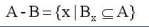
该公式表示图像A用卷积模板B来进行腐蚀处理，通过模板B与图像A进行卷积计算，得出B覆盖区域的像素点最小值，并用这个最小值来替代参考点的像素值。

把结构元素B平移a后得到Ba，若Ba包含于X，我们记下这个a点，所有满足上述条件的a点组成的集合称作X被B腐蚀的结果。如下图所示。其结果像X被拨掉了周围一层。
在这里插入图片描述
举例说明：

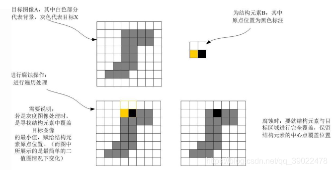
上图中结构元素B只有下面一行为1，故可理解成1行2列的结构元素。结构元素B中黑色标注的点为原点，当原点滑到前景目标图像A（即图中阴影部分）上时开始腐蚀处理，将B与A重叠部分的像素最小值赋给原点所在位置的A的像素点。随后继续滑动，直到滑过整幅图片。
示例腐蚀结果如下：
在这里插入图片描述
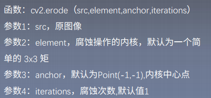
腐蚀操作在opencv中的函数如下：

import cv2
import numpy as np 
import matplotlib.pyplot as plt
img = cv2.imread('./image/morphology.png')
img = cv2.cvtColor(img,cv2.COLOR_BGR2RGB)
kernel = np.ones((3,3),np.uint8)
#kernel = np.ones((5,5),np.uint8)
#kernel = cv2.getStructuringElement(cv2.MORPH_CROSS, (7,7))
#kernel = cv2.getStructuringElement(cv2.MORPH_ELLIPSE, (7,7))
#kernel = cv2.getStructuringElement(cv2.MORPH_RECT, (7,7))
#print(kernel)
erosion = cv2.erode(img,kernel,iterations = 1)
#eroded = cv2.erode(gray.copy(), kernel, 10)
# eroded = cv2.erode(gray.copy(), None, 10)
plt.subplot(121),plt.imshow(img),plt.title('Original')
plt.xticks([]), plt.yticks([])
plt.subplot(122),plt.imshow(erosion),plt.title('erosion')
plt.xticks([]), plt.yticks([])
plt.show()

运行结果：
在这里插入图片描述

2.图像膨胀
膨胀类似于“领域扩张”，将图像中的白色部分进行扩张，其运行结果图比原图的白色区域更大。
理解腐蚀以后对于膨胀则很容易理解。下面通过示例说明：
在这里插入图片描述
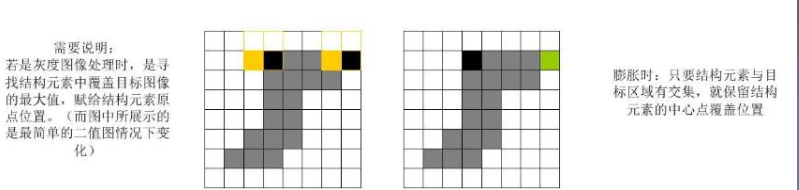
**注：**膨胀时，只要结构元素与目标区域有交集即开始处理，而腐蚀必须要结构元素的原点与目标区域有交集才可。两者也有相同之处，即始终是对结构元素B的原点所在位置进行操作。
示例膨胀后的图像为：
在这里插入图片描述

import cv2 
import numpy as np
import matplotlib.pyplot as plt
img = cv2.imread('./image/morphology.png')
img = cv2.cvtColor(img,cv2.COLOR_BGR2RGB)
#kernel = np.ones((3,),np.uint8)
kernel = cv2.getStructuringElement(cv2.MORPH_RECT, (7,7))

dilation = cv2.dilate(img,kernel,iterations = 1)
kernel1 = np.ones((7,7),np.uint8)
opening = cv2.morphologyEx(dilation,cv2.MORPH_OPEN,kernel1)
plt.subplot(121),plt.imshow(opening),plt.title('opening')
plt.xticks([]), plt.yticks([])
plt.subplot(122),plt.imshow(dilation),plt.title('dilation')
plt.xticks([]), plt.yticks([])
plt.show()

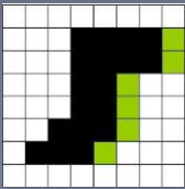
3.开运算
开运算，即先腐蚀再膨胀，它能够去除孤立的小点，毛刺和小桥，而总的位置和形状不变。
在这里插入图片描述

import cv2
import numpy as np
import matplotlib.pyplot as plt
img = cv2.imread('./image/open.png')
img = cv2.cvtColor(img,cv2.COLOR_BGR2RGB)
#kernel = np.ones((5,5),np.uint8)
kernel = cv2.getStructuringElement(cv2.MORPH_RECT, (9,9))
opening = cv2.morphologyEx(img,cv2.MORPH_OPEN,kernel)
plt.subplot(121),plt.imshow(img),plt.title('Original')
plt.xticks([]), plt.yticks([])
plt.subplot(122),plt.imshow(opening),plt.title('opening')
plt.xticks([]), plt.yticks([])
plt.show()

4.闭运算
闭运算，即先膨胀再腐蚀。闭运算能够填平小孔，弥合小裂缝，而总的位置和形状不变。
在这里插入图片描述

import cv2 as cv
import numpy as np
img = cv.imread('./image/close.png')
img = cv.cvtColor(img,cv.COLOR_BGR2RGB)
#kernel = np.ones((5,5),np.uint8)
kernel = np.ones((7,7),np.uint8)
closing = cv.morphologyEx(img,cv.MORPH_CLOSE,kernel)
plt.subplot(121),plt.imshow(img),plt.title('Original')
plt.xticks([]), plt.yticks([])
plt.subplot(122),plt.imshow(closing),plt.title('closing')
plt.xticks([]), plt.yticks([])
plt.show()

5.形态学梯度（Gradient）
基础梯度 = 膨胀图 - 腐蚀图
内部梯度 = 原图 - 腐蚀图
外部梯度 = 膨胀 - 原图

import cv2 as cv
import numpy as np
import matplotlib.pyplot as plt
img = cv.imread('./image/morphology.png')
img = cv.cvtColor(img,cv.COLOR_BGR2RGB)
kernel = np.ones((3,3),np.uint8)
gradient = cv.morphologyEx(img,cv.MORPH_GRADIENT,kernel)
plt.subplot(121),plt.imshow(img),plt.title('Original')
plt.xticks([]), plt.yticks([])
plt.subplot(122),plt.imshow(gradient),plt.title('gradient')
plt.xticks([]), plt.yticks([])
plt.show()

6.顶帽和黑帽
顶帽：原图 - 开运算图，突出源图像中比周围亮的区域
黑帽：闭运算图 - 原图，突出原图像中比周围暗的区域

#顶帽：示例针对9x9内核完成
import cv2 as cv
import numpy as np
import matplotlib.pyplot as plt
img = cv.imread('./image/morphology.png')
img = cv.cvtColor(img,cv.COLOR_BGR2RGB)
kernel = np.ones((9,9),np.uint8)
tophat = cv.morphologyEx(img,cv.MORPH_TOPHAT,kernel)
plt.subplot(121),plt.imshow(img),plt.title('Original')
plt.xticks([]), plt.yticks([])
plt.subplot(122),plt.imshow(tophat),plt.title('tophat')
plt.xticks([]), plt.yticks([])
plt.show()

#黑帽
tophat = cv.morphologyEx(img,cv.MORPH_BLACKHAT,kernel)

3.图像分割与代码实现

3.1 图像分割概念

图像分割是指将图像分成若干具有相似性质的区域的过程，主要有基于阈值、基于区域、基于边缘、基于聚类、基于图论和基于深度学习的图像分割方法。分割的原则是使划分后的子图在内部保持相似度最大，而子图之间的相似度保持最小。
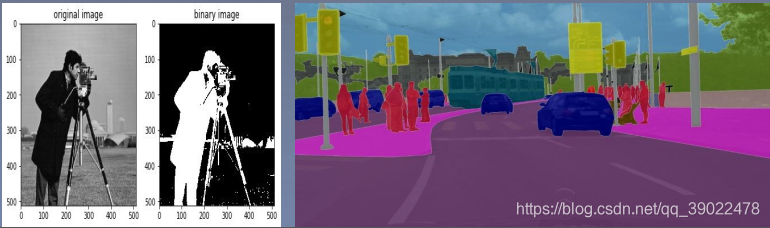
图像分割分为语义分割（下图左）和实例分割（下图右）。
在这里插入图片描述

3.2 固定阈值法

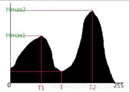
1.直方图双峰法
这是一种典型的全局单阈值分割方法。如下图所示，算法基本思想是：假设图像中有明显的目标和背景，则其灰度直方图成双峰分布，当灰度级直方图具有双峰特性时，选取双峰之间的谷对应的灰度级作为阈值。
在这里插入图片描述
固定阈值分割在opencv中的函数为：

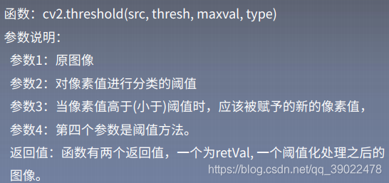
可根据参数4来设置参数3的值，而参数4的阈值方法有以下几种：

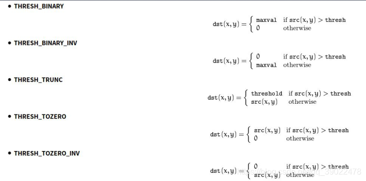
代码实现：固定阈值分割不同方法比较

import cv2
from matplotlib import pyplot as plt
#opencv读取图像 
img = cv2.imread('./image/person.png',0)
#5种阈值法图像分割
ret, thresh1 = cv2.threshold(img, 127, 255, cv2.THRESH_BINARY)
ret, thresh2 = cv2.threshold(img, 127, 255, cv2.THRESH_BINARY_INV)
ret, thresh3 = cv2.threshold(img, 127, 255,cv2.THRESH_TRUNC)
ret, thresh4 = cv2.threshold(img, 127, 255, cv2.THRESH_TOZERO)
ret, thresh5 = cv2.threshold(img, 127, 255, cv2.THRESH_TOZERO_INV)

images = [img, thresh1, thresh2, thresh3, thresh4, thresh5]
#使用for循环进行遍历，matplotlib进行显示
for i in range(6):
    plt.subplot(2,3, i+1)
    plt.imshow(images[i],cmap='gray')
    plt.xticks([])
    plt.yticks([])

plt.suptitle('fixed threshold')
plt.show()

运行结果：
在这里插入图片描述

3.3 自动阈值法

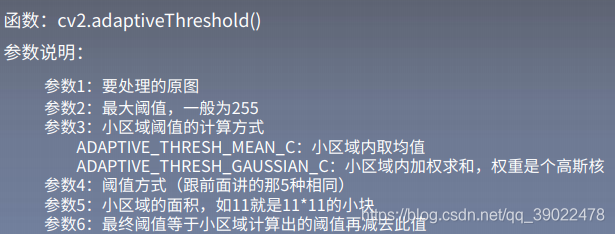
1.自适应阈值法
该方法特点是每次取图片的一小部分计算阈值，这样图片不同区域的阈值就不尽相同，适用于明暗分布不均的图片。
在这里插入图片描述
代码：自适应阈值与固定阈值对比

import cv2
import matplotlib.pyplot as plt
img = cv2.imread('./image/paper2.png', 0)

# 固定阈值
ret, th1 = cv2.threshold(img, 127, 255, cv2.THRESH_BINARY)
# 自适应阈值
th2 = cv2.adaptiveThreshold(
    img, 255, cv2.ADAPTIVE_THRESH_MEAN_C, cv2.THRESH_BINARY,11, 4)
th3 = cv2.adaptiveThreshold(
    img, 255, cv2.ADAPTIVE_THRESH_GAUSSIAN_C, cv2.THRESH_BINARY, 11, 4)
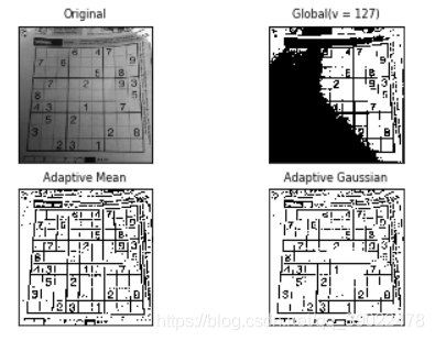
#全局阈值，均值自适应，高斯加权自适应对比
titles = ['Original', 'Global(v = 127)', 'Adaptive Mean', 'Adaptive Gaussian']
images = [img, th1, th2, th3]
for i in range(4):
    plt.subplot(2, 2, i + 1), plt.imshow(images[i], 'gray')
    plt.title(titles[i], fontsize=8)
    plt.xticks([]), plt.yticks([])
plt.show()

运行结果：
在这里插入图片描述
2.迭代法阈值分割
步骤：

求出图像的最大灰度值和最小灰度值，分别记为ZMAX和ZMIN，令初始阈值为T0=（ZMAX+ZMIN)/2;
根据阈值Tk将图像分割为前景和背景，分别求出两者的平均灰度值ZO和ZB；
求出新阈值Tk+1 = （ZO+ZB)/2;
若Tk==Tk+1，则所得即为阈值；否则进行步骤2，迭代计算；
使用计算后的阈值进行固定阈值分割。

代码：迭代法

#import tensorflow as tf
import cv2
import numpy as np
import matplotlib.pyplot as plt
import matplotlib.cm as cm

def best_thresh(img):
    img_array = np.array(img).astype(np.float32)#转化成数组
    I=img_array
    zmax=np.max(I)
    zmin=np.min(I)
    tk=(zmax+zmin)/2#设置初始阈值
    #根据阈值将图像进行分割为前景和背景，分别求出两者的平均灰度zo和zb
    b=1
    m,n=I.shape;
    while b==0:
        ifg=0
        ibg=0
        fnum=0
        bnum=0
        for i in range(1,m):
             for j in range(1,n):
                tmp=I(i,j)
                if tmp>=tk:
                    ifg=ifg+1
                    fnum=fnum+int(tmp)#前景像素的个数以及像素值的总和
                else:
                    ibg=ibg+1
                    bnum=bnum+int(tmp)#背景像素的个数以及像素值的总和
        #计算前景和背景的平均值
        zo=int(fnum/ifg)
        zb=int(bnum/ibg)
        if tk==int((zo+zb)/2):
            b=0
        else:
            tk=int((zo+zb)/2)
    return tk

img = cv2.imread("./image/bird.png")
img = cv2.cvtColor(img,cv2.COLOR_BGR2RGB)
gray = cv2.cvtColor(img,cv2.COLOR_RGB2GRAY)
img = cv2.resize(gray,(200,200))#大小
yvzhi=best_thresh(img)
ret1, th1 = cv2.threshold(img, yvzhi, 255, cv2.THRESH_BINARY)
print(ret1)
plt.imshow(th1,cmap=cm.gray)
plt.show()

3.Otsu大津法
大津法即最大类间差法，1979年由日本学者大津提出，是一种基于全局阈值的自适应方法。当取最佳阈值时，图像前景和背景之间的差别应该是最大的，衡量差别的标准为最大类间方差。如果直方图有两个峰值的图像，大津法求得的T近似等于两个峰值之间的低谷。
当取阈值为T时，图像类间方差g的计算公式如下：
在这里插入图片描述
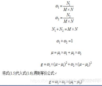
其中：w1：属于前景的像素点数占整幅图像的比例，其平均灰度为u1；w2：属于背景的像素点数占整幅图像的比例，其平均灰度为u2；u：图像的总平均灰度；N1：设图像大小为M*N,图像中像素的灰度值小于阈值T的像素个数；N2：像素灰度大于阈值T的像素个数。

代码：固定阈值、大津、高斯滤波+大津方法比较

import cv2
from matplotlib import pyplot as plt
img = cv2.imread('./image/noisy.png', 0)
# 固定阈值法
ret1, th1 = cv2.threshold(img, 100, 255, cv2.THRESH_BINARY)
# Otsu阈值法
ret2, th2 = cv2.threshold(img, 0, 255, cv2.THRESH_BINARY + cv2.THRESH_OTSU)

# 先进行高斯滤波，再使用Otsu阈值法
blur = cv2.GaussianBlur(img, (5, 5), 0)
ret3, th3 = cv2.threshold(blur, 0, 255, cv2.THRESH_BINARY + cv2.THRESH_OTSU)
images = [img, 0, th1, img, 0, th2, blur, 0, th3]
titles = ['Original', 'Histogram', 'Global(v=100)',
         'Original', 'Histogram', "Otsu's",
         'Gaussian filtered Image', 'Histogram', "Otsu's"]

for i in range(3):
    # 绘制原图
    plt.subplot(3, 3, i * 3 + 1)
    plt.imshow(images[i * 3], 'gray')
    plt.title(titles[i * 3], fontsize=8)
    plt.xticks([]), plt.yticks([])
    
    # 绘制直方图plt.hist, ravel函数将数组降成一维
    plt.subplot(3, 3, i * 3 + 2)
    plt.hist(images[i * 3].ravel(), 256)
    plt.title(titles[i * 3 + 1], fontsize=8)
    plt.xticks([]), plt.yticks([])
    
    # 绘制阈值图
    plt.subplot(3, 3, i * 3 + 3)
    plt.imshow(images[i * 3 + 2], 'gray')
    plt.title(titles[i * 3 + 2], fontsize=8)
    plt.xticks([]), plt.yticks([])
plt.show()

运行结果：
在这里插入图片描述
代码：Ostu源码

import numpy as np
 
def OTSU_enhance(img_gray, th_begin=0, th_end=256, th_step=1):
    #"must input a gary_img"
    assert img_gray.ndim == 2
 
    max_g = 0
    suitable_th = 0
    for threshold in range(th_begin, th_end, th_step):
        bin_img = img_gray > threshold
        bin_img_inv = img_gray <= threshold
        fore_pix = np.sum(bin_img)
        back_pix = np.sum(bin_img_inv)
        if 0 == fore_pix:
            break
        if 0 == back_pix:
            continue
 
        w0 = float(fore_pix) / img_gray.size
        u0 = float(np.sum(img_gray * bin_img)) / fore_pix
        w1 = float(back_pix) / img_gray.size
        u1 = float(np.sum(img_gray * bin_img_inv)) / back_pix
        # intra-class variance
        g = w0 * w1 * (u0 - u1) * (u0 - u1)
        if g > max_g:
            max_g = g
            suitable_th = threshold
    return suitable_th
img = cv2.imread('noisy.png', 0)
thresh = OTSU_enhance(img)
ret1, th1 = cv2.threshold(img, thresh, 255, cv2.THRESH_BINARY)
ret2, th2 = cv2.threshold(img, 0, 255, cv2.THRESH_BINARY+cv2.THRESH_OTSU)
a = plt.imshow(th1,cmap=cm.gray)
plt.show(a)
b = plt.imshow(th2,cmap=cm.gray)
plt.show(b)

3.4 边缘检测/提取

1.梯度
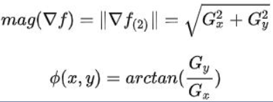
梯度是一个向量，方向为函数变化最快的方向，大小等于该向量的模长，也是最大的变化率。对于二元函数z=f(x,y),它在点（x,y)的梯度就是gradf(x,y).
在这里插入图片描述
这个梯度向量的幅度和方向角为：

2.图像梯度
图像梯度即图像中灰度变化的度量，求图像梯度的过程是二维离散函数求导过程。边缘可理解为图像上灰度变化较快的点的集合。
对于像素点（x,y),它的灰度值为f(x,y),它有八个邻域：
在这里插入图片描述
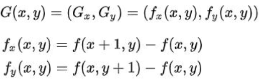
图像在点（x,y)的梯度为：

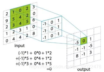
3.模板卷积
模板卷积步骤如下：

将模板在输入图像中滑动，使得模板中心与图像中某个像素位置重合；
将模板上各个系数与模板下各对应像素的灰度相乘；
将所有乘积相加（为保持灰度范围，常将结果再除以模板系数之和，后面梯度算子模板和为0的话就不需要除了）；
将上述运算结果（模板的相应输出）赋给图像中对应模板中心位置的像素。

4.梯度图
梯度图的生成和模板卷积相同，不同的是要生成梯度图，还需要在模板卷积完成后计算在点（x,y)梯度的幅值，将幅值作为像素值，才算结束。

**注：**梯度图上每个像素点的灰度值就是梯度向量的幅度。
生成梯度图需要模板，下图为水平和竖直方向最简单的模板:
水平方向：g(x,y)=|G(x)|=|f(x+1,y)-f(x,y)|

在这里插入图片描述
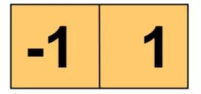
竖直方向：g(x,y)=|G(y)|=|f(x,y+1)-f(x,y)|

5.梯度算子
梯度算子是一阶导数算子，是水平G(x)和竖直G(y)方向对应模板的组合，也有对角线方向。
常见一阶算子：roberts交叉算子，sobel算子

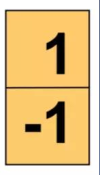
Roberts交叉算子：
在这里插入图片描述
该算子本质上是一个对角线方向的梯度算子，对应的水平方向和竖直方向的梯度分别为：
Gx = f(x+1,y+1) - f(x,y)
Gy = f(x,y+1) - f(x+1,y)
优点：边缘定位较准，适用于边缘明显且噪声较少的图像；
缺点：1.没有描述水平和竖直方向的灰度变化，只关注了对角线方向；2.鲁棒性差。由于本身参加了梯度计算，不能有效地抑制噪声的干扰。

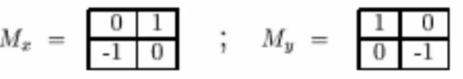
Sobel算子：
在这里插入图片描述
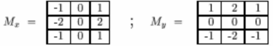
sobel算子其实就是增加了权重系数的prewitt算子，故这里只介绍sobel。该模板中心对应原图坐标点的8-邻域像素灰度值如下所示：

过sobel算子的水平模板Mx卷积后，对应的水平方向梯度为：
Gx = f(x+1,y+1)-f(x-1,y+1)+2f(x+1,y)-2f(x-1,y)+f(x+1,y-1)-f(x-1,y-1)
过sobel算子的竖直模板Mx卷积后，对应的竖直方向梯度为：
Gy = f(x-1,y+1)-f(x-1,y-1)+2f(x,y-1)-2f(x,y-1)+f(x+1,y+1)-f(x+1,y-1)
输出梯度图在(x,y)的灰度值为 $\sqrt{(G_x^2 + G_y^2)}$ .

sobel算子较为常用，opencv中的相应函数如下：
在这里插入图片描述

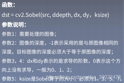
import numpy as np
import cv2
from matplotlib import pyplot as plt
img = cv2.imread('image/girl2.png',0)
sobelx = cv2.Sobel(img,cv2.CV_64F,1,0,ksize=5)
sobely = cv2.Sobel(img,cv2.CV_64F,0,1,ksize=5)



plt.subplot(1,3,1),plt.imshow(img,cmap = 'gray')
plt.title('Original'), plt.xticks([]), plt.yticks([])
plt.subplot(1,3,2),plt.imshow(sobelx,cmap = 'gray')
plt.title('Sobel X'), plt.xticks([]), plt.yticks([])
plt.subplot(1,3,3),plt.imshow(sobely,cmap = 'gray')
plt.title('Sobel Y'), plt.xticks([]), plt.yticks([])
plt.show()

6.Canny边缘检测算法
Canny算子是先平滑后求导数的方法。该算法有较好的错判率，定位性能，且对单一边缘仅有唯一响应。
算法步骤如下：

彩色图像转换为灰度图（以灰度图单通道读入）；
对图像进行高斯模糊（去噪）；
计算图像梯度，根据梯度计算图像边缘幅值与角度；
沿梯度方向进行非极大值抑制（边缘细化）；
双阈值边缘连接处理；
二值化图像输出结果

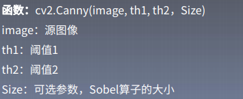
代码：

import cv2
import numpy as np
#以灰度图形式读入图像
img = cv2.imread('image/canny.png')
v1 = cv2.Canny(img, 80, 150,(3,3))
v2 = cv2.Canny(img, 50, 100,(5,5))

#np.vstack():在竖直方向上堆叠
#np.hstack():在水平方向上平铺堆叠
ret = np.hstack((v1, v2))
cv2.imshow('img', ret)
cv2.waitKey(0)
cv2.destroyAllWindows()

3.5 连通区域分析

连通区域（connected component）一般是指图像中具有相同像素值且位置相邻的前景像素点组成的图像区域，连通区域分析是指将图像中的各个连通区域找出并标记。连通区域分析是一种在CV和图像分析处理的众多应用领域中较为常用和基本的方法。
在需要将前景目标提取出来以便后续处理的应用场景中都能够用到连通区域分析方法，通常连通区域分析处理的对象是一张二值化后的图像
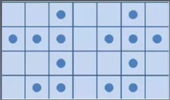
常见的邻接关系有两种：4邻接（下图左）和8邻接（下图右）。
在这里插入图片描述
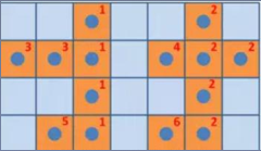
Two-Pass算法：
该算法通过扫描两遍图像，将图像中存在的所有连通域找出并标记：
第一次扫描：从左上角开始遍历像素点，找到第一个像素为255的点，label=1；当该像素的左邻像素或者上邻像素为无效值时，给该像素设置一个新的label值，label++，记录集合；当该像素的左邻像素或者上邻像素有一个为有效值时，将有效值像素的label赋给该像素的label值；当该像素的左邻像素和上邻像素都为有效值时，选取其中较小的label值赋给该像素的label值。
第二次扫描：对每个点的label进行更新，更新为其对于其集合中最小的label。
原图：
在这里插入图片描述
第一次扫描后：

第二次扫描后：

代码实现：

import cv2
import numpy as np

# 4邻域的连通域和 8邻域的连通域
# [row, col]
NEIGHBOR_HOODS_4 = True
OFFSETS_4 = [[0, -1], [-1, 0], [0, 0], [1, 0], [0, 1]]

NEIGHBOR_HOODS_8 = False
OFFSETS_8 = [[-1, -1], [0, -1], [1, -1],
             [-1,  0], [0,  0], [1,  0],
             [-1,  1], [0,  1], [1,  1]]

def reorganize(binary_img: np.array):
    index_map = []
    points = []
    index = -1
    rows, cols = binary_img.shape
    for row in range(rows):
        for col in range(cols):
            var = binary_img[row][col]
            if var < 0.5:
                continue
            if var in index_map:
                index = index_map.index(var)
                num = index + 1
            else:
                index = len(index_map)
                num = index + 1
                index_map.append(var)
                points.append([])
            binary_img[row][col] = num
            points[index].append([row, col])
    return binary_img, points

def neighbor_value(binary_img: np.array, offsets, reverse=False):
    rows, cols = binary_img.shape
    label_idx = 0
    rows_ = [0, rows, 1] if reverse == False else [rows-1, -1, -1]
    cols_ = [0, cols, 1] if reverse == False else [cols-1, -1, -1]
    for row in range(rows_[0], rows_[1], rows_[2]):
        for col in range(cols_[0], cols_[1], cols_[2]):
            label = 256
            if binary_img[row][col] < 0.5:
                continue
            for offset in offsets:
                neighbor_row = min(max(0, row+offset[0]), rows-1)
                neighbor_col = min(max(0, col+offset[1]), cols-1)
                neighbor_val = binary_img[neighbor_row, neighbor_col]
                if neighbor_val < 0.5:
                    continue
                label = neighbor_val if neighbor_val < label else label
            if label == 255:
                label_idx += 1
                label = label_idx
            binary_img[row][col] = label
    return binary_img

# binary_img: bg-0, object-255; int
def Two_Pass(binary_img: np.array, neighbor_hoods):
    if neighbor_hoods == NEIGHBOR_HOODS_4:
        offsets = OFFSETS_4
    elif neighbor_hoods == NEIGHBOR_HOODS_8:
        offsets = OFFSETS_8
    else:
        raise ValueError

    binary_img = neighbor_value(binary_img, offsets, False)
    binary_img = neighbor_value(binary_img, offsets, True)

    return binary_img

if __name__ == "__main__":
    binary_img = np.zeros((4, 7), dtype=np.int16)
    index = [[0, 2], [0, 5],
            [1, 0], [1, 1], [1, 2], [1, 4], [1, 5], [1, 6],
            [2, 2], [2, 5],
            [3, 1], [3, 2], [3, 4],[3,5], [3, 6]]
    for i in index:
        binary_img[i[0], i[1]] = np.int16(255)

    print("原始二值图像")
    print(binary_img)

    print("Two_Pass")
    binary_img = Two_Pass(binary_img, NEIGHBOR_HOODS_4)
    binary_img, points = reorganize(binary_img)
    print(binary_img)
    #print(points)

3.6 区域生长算法

区域生长是指从某个像素出发，按照一定的准则，逐步加入邻近像素，当满足一定的条件时，区域生长终止。进而实现目标的提取。
区域生长的好坏决定于：初始点的选取，生长条件，终止条件。
算法步骤：

对图像顺序扫描，找到第一个还没有归属的像素，设该像素为(x0,y0);
以(x0,y0)为中心，考虑其4邻域像素(x,y),若满足生长条件，则将(x,y)与(x0,y0)合并（在同一区域内），同时将(x,y)压入堆栈；
从堆栈中取出一个像素，把它当作(x0,y0)返回步骤2；
当堆栈为空时，返回步骤1；
重复步骤1-4直到图像中的每个点都有归属时，生长结束。

代码1：

import cv2
import numpy as np
from matplotlib import pyplot as plt
import sys
def on_mouse(event, x, y, flags, params):
    if event == cv2.EVENT_LBUTTONDOWN:
        print ('Start Mouse Position: ' + str(x) + ', ' + str(y))
        s_box = x, y
        print(s_box)
        boxes.append(s_box)

def region_growing(img, seed):
    #Parameters for region growing
    neighbors = [(-1, 0), (1, 0), (0, -1), (0, 1)]
    region_threshold = 0.2
    region_size = 1
    intensity_difference = 0
    neighbor_points_list = []
    neighbor_intensity_list = []

    #Mean of the segmented region
    region_mean = img[seed]

    #Input image parameters
    height, width = img.shape
    image_size = height * width

    #Initialize segmented output image
    segmented_img = np.zeros((height, width, 1), np.uint8)

    #Region growing until intensity difference becomes greater than certain threshold
    while (intensity_difference < region_threshold) & (region_size < image_size):
        #Loop through neighbor pixels
        for i in range(4):
            #Compute the neighbor pixel position
            x_new = seed[0] + neighbors[i][0]
            y_new = seed[1] + neighbors[i][1]

            #Boundary Condition - check if the coordinates are inside the image
            check_inside = (x_new >= 0) & (y_new >= 0) & (x_new < height) & (y_new < width)

            #Add neighbor if inside and not already in segmented_img
            if check_inside:
                if segmented_img[x_new, y_new] == 0:
                    neighbor_points_list.append([x_new, y_new])
                    neighbor_intensity_list.append(img[x_new, y_new])
                    segmented_img[x_new, y_new] = 255

        #Add pixel with intensity nearest to the mean to the region
        distance = abs(neighbor_intensity_list-region_mean)
        pixel_distance = min(distance)
        index = np.where(distance == pixel_distance)[0][0]
        segmented_img[seed[0], seed[1]] = 255
        region_size += 1

        #New region mean
        region_mean = (region_mean*region_size + neighbor_intensity_list[index])/(region_size+1)

        #Update the seed value
        seed = neighbor_points_list[index]
        #Remove the value from the neighborhood lists
        neighbor_intensity_list[index] = neighbor_intensity_list[-1]
        neighbor_points_list[index] = neighbor_points_list[-1]

    return segmented_img


if __name__ == '__main__':

    boxes = []
    filename = 'image/region_grow.jpg'
    img = cv2.imread(filename, 0)
    resized = cv2.resize(img,(256,256))
    cv2.namedWindow('input')
    cv2.setMouseCallback('input', on_mouse, 0,)
    cv2.imshow('input', resized)
    cv2.waitKey(0)
    print('boxes::::',boxes)
    print ("Starting region growing based on last click")
    seed = boxes[-1]
    print("seed:::::",seed)
    output = region_growing(resized, seed)
    
    print ("Done. Showing output now")
    cv2.imshow('output',output )
    cv2.waitKey(0)
    cv2.destroyAllWindows()

代码2：

# -*- coding:utf-8 -*-
import cv2
import numpy as np

####################################################################################

#import Image
im = cv2.imread('image/222.jpg')
im_shape = im.shape
height = im_shape[0]
width = im_shape[1]

print( 'the shape of image :', im_shape)

#######################################################################################
class Point(object):
    def __init__(self , x , y):
        self.x = x
        self.y = y
    def getX(self):
        return self.x
    def getY(self):
        return self.y
connects = [ Point(-1, -1), Point(0, -1), Point(1, -1), Point(1, 0), Point(1, 1), Point(0, 1), Point(-1, 1), Point(-1, 0)]
#####################################################################################
#计算两个点间的欧式距离
def get_dist(seed_location1,seed_location2):
    l1 = im[seed_location1.x , seed_location1.y]
    l2 = im[seed_location2.x , seed_location2.y]
    count = np.sqrt(np.sum(np.square(l1-l2)))
    return count
########################################################################################
def on_mouse(event, x, y, flags, params):
    s_box = []
    if event == cv2.EVENT_LBUTTONDOWN:
        print ('Start Mouse Position: ' + str(x) + ', ' + str(y))
        p_box =[x, y]
        s_box,append(p_box)


#标记，判断种子是否已经生长
img_mark = np.zeros([height , width])

# 建立空的图像数组,作为一类
img_re = im.copy()
for i in range(height):
    for j in range(width):
        img_re[i, j][0] = 0
        img_re[i, j][1] = 0
        img_re[i, j][2] = 0
#随即取一点作为种子点
seed_list = []
seed_list.append(Point(15, 15))
T = 7#阈值
class_k = 1#类别
#生长一个类
while (len(seed_list) > 0):
    seed_tmp = seed_list[0]
    #将以生长的点从一个类的种子点列表中删除
    seed_list.pop(0)


    img_mark[seed_tmp.x, seed_tmp.y] = class_k

    # 遍历8邻域
    for i in range(8):
        tmpX = seed_tmp.x + connects[i].x
        tmpY = seed_tmp.y + connects[i].y

        if (tmpX < 0 or tmpY < 0 or tmpX >= height or tmpY >= width):
            continue
        dist = get_dist(seed_tmp, Point(tmpX, tmpY))
        #在种子集合中满足条件的点进行生长
        if (dist < T and img_mark[tmpX, tmpY] == 0):
            img_re[tmpX, tmpY][0] = im[tmpX, tmpY][0]
            img_re[tmpX, tmpY][1] = im[tmpX, tmpY][1]
            img_re[tmpX, tmpY][2] = im[tmpX, tmpY][2]
            img_mark[tmpX, tmpY] = class_k
            seed_list.append(Point(tmpX, tmpY))


########################################################################################

#输出图像
cv2.imshow('OUTIMAGE' , img_re)
cv2.waitKey(0)
cv2.destroyAllWindows()

补充：opencv鼠标操作示例代码

import cv2
import numpy as np 
import time
 
img=cv2.imread('image/222.jpg') #读取图片作为背景
 
#定义画圆事件，如果事件双击左键发生
#则以此时双击的点为原点画一个半径为100px BGR为(255,255,0)粗细为3px的圆圈
def draw_circle(event,x,y,flags,param): 
	
	if event==cv2.EVENT_LBUTTONDBLCLK:
		cv2.circle(img,(x,y),100,(255,255,0),3)
		
# 创建图像与窗口并将窗口与回调函数绑定
cv2.namedWindow('image') 
cv2.setMouseCallback('image',draw_circle)
 
while(1):
	cv2.imshow('image',img)
	if cv2.waitKey(100) == ord('q'):	#等待100毫秒 刷新一次显示图像
		break
cv2.destroyAllWindows()

4.图像特征提取与代码实现

4.1 图像特征理解

图像特征是图像中独特的，易于跟踪和比较的特定模板或特定结构。如下图中E等。
在这里插入图片描述
图像特征主要有图像的颜色特征、纹理特征、形状特征和空间关系特征。

1.颜色特征
颜色特征是一种全局特征，描述了图像或图像区域所对应的景物的表面性质。
颜色特征描述方法：颜色直方图；颜色空间；颜色分布

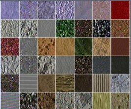
2.纹理特征
纹理特征也是一种全局特征，它也描述了图像或图像区域所对应景物的表面性质。但由于纹理只是一种物体表面的特性，并不能完全反映出物体的本质属性，所以仅仅利用纹理特征是无法获得高层次图像内容的。
在这里插入图片描述
3.形状特征
形状特征有两类表示方法，一类是轮廓特征，主要针对物体的外边界；另一类是区域特征，描述了图像中的局部形状特征。

4.空间关系特征
指图像中分割出来的多个目标之间的相互的空间位置或相对方向关系。这些关系也可分为连接/邻接关系，交叠/重叠关系和包含/独立关系等。
在这里插入图片描述

4.2 形状特征

4.2.1 Hog特征提取

方向梯度直方图（Histogram of Oriented Gradient, HOG)特征是一种用来进行物体检测的特征描述子，它通过计算和统计图像局部区域的梯度方向直方图来构成特征。Hog特征结合SVM分类器在图像识别、行人检测中应用广泛。Hog特征提取的主要思想是：在一幅图像中，目标的形状能够被梯度或边缘的方向密度分布很好的描述。

HOG实现过程：

灰度化（将图象看作一个x,y,z(灰度)的三维图像）；
采用Gamma校正法对输入图像进行颜色空间的标准化（归一化）；
计算图像每个像素的梯度（包括大小和方向）；
将图像划分成小cells；
统计每个cell的梯度直方图（不同梯度的个数），得到cell的描述子；
将每几个cell组成一个block，得到block的描述子；
将图像image内的所有block的HOG特征descriptor串联起来就可以得到Hog特征，该特征向量就是用来目标检测或分类的特征。

代码：Hog特征

import cv2
import numpy as np
# 判断矩形i是否完全包含在矩形o中
def is_inside(o, i):
    ox, oy, ow, oh = o
    ix, iy, iw, ih = i
    return ox > ix and oy > iy and ox + ow < ix + iw and oy + oh < iy + ih
# 对人体绘制颜色框
def draw_person(image, person):
    x, y, w, h = person
    cv2.rectangle(image, (x, y), (x + w, y + h), (0, 255, 255), 2)
img = cv2.imread("people.jpg")
hog = cv2.HOGDescriptor()  # 启动检测器对象
hog.setSVMDetector(cv2.HOGDescriptor_getDefaultPeopleDetector())  # 指定检测器类型为人体
found, w = hog.detectMultiScale(img,0.1,(2,2)) # 加载并检测图像
print(found)
print(w)

# 丢弃某些完全被其它矩形包含在内的矩形
found_filtered = []
for ri, r in enumerate(found):
    for qi, q in enumerate(found):
        if ri != qi and is_inside(r, q):
            break
    else:
        found_filtered.append(r)
        print(found_filtered)
# 对不包含在内的有效矩形进行颜色框定
for person in found_filtered:
    draw_person(img, person)
cv2.imshow("people detection", img)
cv2.waitKey(0)
cv2.destroyAllWindows()

4.2.2 Harris角点检测

1.角点
现实世界中，角点对应于物体的拐角。图像角度来看，角点可以是两个边缘的交点或者是邻域内具有两个主方向的特征点，相应于计算方法上，前者通过图像边缘计算，计算量大，图像局部变化会对结果产生较大的影响；后者基于图像灰度的方法通过计算点的曲率及梯度来检测角点。
对于同一场景，即使视角发生变化，角点仍具有较为稳定的性质。所以角点适用于图像的定位等方面。

Harris实现过程：
1.计算图像在X和Y方向的梯度：
在这里插入图片描述
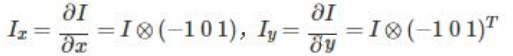
2.计算图像两个方向梯度的乘积；

3.使用高斯函数对三者进行高斯加权，生成矩阵M的A,B,C;

4.计算每个像素的Harris响应值R，并对小于某一阈值T的R置为零；
5.在33或55的邻域内进行非最大值抑制，局部最大点即为图像中的角点。

代码实现：

import cv2
import numpy as np
from matplotlib import pyplot as plt

img = cv2.imread('harris2.png')
img = cv2.cvtColor(img, cv2.COLOR_BGR2RGB)
gray = cv2.cvtColor(img, cv2.COLOR_BGR2GRAY)
gray = np.float32(gray)
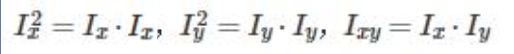
dst_block9_ksize19 = cv2.cornerHarris(gray, 9, 19, 0.04)
img1 = np.copy(img)
img1[dst_block9_ksize19 > 0.01 * dst_block9_ksize19.max()] = [0, 0, 255]

dst_block5_ksize19 = cv2.cornerHarris(gray, 5, 19, 0.04)
img2 = np.copy(img)
img2[dst_block5_ksize19 > 0.01 * dst_block5_ksize19.max()] = [0, 0, 255]

dst_block9_ksize5 = cv2.cornerHarris(gray, 9, 5, 0.04)
img3 = np.copy(img)
img3[dst_block9_ksize5 > 0.01 * dst_block9_ksize5.max()] = [0, 0, 255]

dst_block9_ksize31 = cv2.cornerHarris(gray, 9, 31, 0.04)
img4 = np.copy(img)
img4[dst_block9_ksize31 > 0.01 * dst_block9_ksize31.max()] = [0, 0, 255]

dst_block9_ksize19_k6 = cv2.cornerHarris(gray, 9, 19, 0.06)
img5 = np.copy(img)
img5[dst_block9_ksize19_k6 > 0.01 * dst_block9_ksize19_k6.max()] = [0, 0, 255]

dst_block9_ksize19_k6_1e_5 = cv2.cornerHarris(gray, 9, 19, 0.06)
img6 = np.copy(img)
img6[dst_block9_ksize19_k6_1e_5 > 0.00001 * dst_block9_ksize19_k6_1e_5.max()] = [0, 0, 255]

titles = ["Original", "block9_ksize19", "dst_block5_ksize19", "dst_block9_ksize5", "dst_block9_ksize31",
          "dst_block9_ksize19_k6", "dst_block9_ksize19_k6_1e_5"]
imgs = [img, img1, img2, img3, img4, img5, img6]
for i in range(len(titles)):
    plt.subplot(3, 3, i + 1), plt.imshow(imgs[i]), plt.title(titles[i])
    plt.xticks([]), plt.yticks([])
plt.show()
# cv2.imshow('src',img)
# cv2.imshow('dst',img5)
# cv2.waitKey(0)
# cv2.destroyAllWindows()

运行结果:
在这里插入图片描述

4.2.3 SIFT

SIFT,即尺度不变特征变换算法。
算法原理细节可参考：SIFT算法详解
SIFT算法源代码实现可参考我的另一篇博客：SIFT之python实现

opencv库函数代码实现：

import cv2
from matplotlib import pyplot as plt

img1 = cv2.imread('road1.jpg', 0)  # queryImage
img2 = cv2.imread('road2.jpg', 0)  # trainImage
# Initiate SIFT detector
sift = cv2.SIFT()
# find the keypoints and descriptors with SIFT
kp1, des1 = sift.detectAndCompute(img1, None)
kp2, des2 = sift.detectAndCompute(img2, None)
# BFMatcher with default params
bf = cv2.BFMatcher()
matches = bf.knnMatch(des1, des2, k=2)
# Apply ratio test
good = []
for m, n in matches:
    if m.distance < 0.75 * n.distance:
        good.append([m])
# cv2.drawMatchesKnn expects list of lists as matches
img3 = cv2.drawMatchesKnn(img1, kp1, img2, kp2, good, flags=2)
plt.imshow(img3)
plt.show()

4.3 纹理特征 LBP

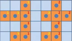
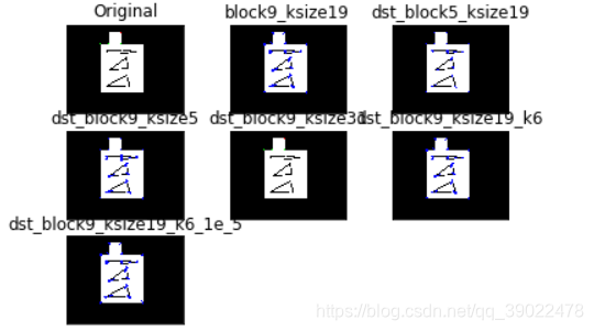
LBP（Local Binary Pattern，局部二值模式），是一种用来描述图像局部纹理特征的算子；它具有旋转不变性和灰度不变性等优点。且LBP记录的是中i性能像素点与邻域像素点之间的差值，所以当光照变化引起像素灰度值同增同减时，LBP也较为稳定。

LBP算子定义在一个3 * 3的窗口内，以窗口中心像素为阈值，与相邻的8个像素的灰度值比较，若周围的像素值大于中心像素值，则该位置被标记为1；否则标记为0.这样可以得到一个8位二进制数（通常还要转换为10进制，即LBP码，共256种），将这个值作为窗口中心像素点的LBP值，以此来反应这个3*3区域的纹理信息。
在这里插入图片描述
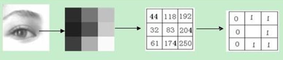
像素顺序从左上角开始顺时针排列，故上图中最后的中心点位置的LBP码为 01111100 = 126

import cv2
import numpy as np
img = cv2.imread('people.jpg',0)
print(img.shape)
def LBP(src):
    '''
    :param src:灰度图像
    :return:
    '''
    height = src.shape[0]
    width = src.shape[1]
    dst = src.copy()
    lbp_value = np.zeros((1,8), dtype=np.uint8)
    #print(lbp_value)
    neighbours = np.zeros((1,8), dtype=np.uint8)
    #print(neighbours)
    for x in range(1, width-1):
        for y in range(1, height-1):
            neighbours[0, 0] = src[y - 1, x - 1]
            neighbours[0, 1] = src[y - 1, x]
            neighbours[0, 2] = src[y - 1, x + 1]
            neighbours[0, 3] = src[y, x - 1]
            neighbours[0, 4] = src[y, x + 1]
            neighbours[0, 5] = src[y + 1, x - 1]
            neighbours[0, 6] = src[y + 1, x]
            neighbours[0, 7] = src[y + 1, x + 1]
            center = src[y, x]
            for i in range(8):
                if neighbours[0, i] > center:
                    lbp_value[0, i] = 1
                else:
                    lbp_value[0, i] = 0

            lbp = lbp_value[0, 0] * 1 + lbp_value[0, 1] * 2 + lbp_value[0, 2] * 4 + lbp_value[0, 3] * 8 \
                + lbp_value[0, 4] * 16 + lbp_value[0, 5] * 32 + lbp_value[0, 6] * 64 + lbp_value[0, 7] * 128
            
            #print(lbp)
            dst[y, x] = lbp

    return dst
new_img = LBP(img)

cv2.imshow('dst',new_img)
cv2.waitKey(0)
cv2.destroyAllWindows()

4.4 模板匹配

简单的说，模板匹配最主要的功能就是在一幅图像中去寻找和另一幅模板图像中相似度最高的部分。通过模板图在目标图上滑动，不断计算匹配程度，匹配最优位置区域即为所求。在opencv中以函数cv2.matchTemplate实现。

matchTemplate(srcImage, templateImage, resultImage, MatchMethod)
参数1: 输入原图像
参数2: 输入模板图像
参数3: 输出的相关系数矩阵
参数4: 匹配方法，有如下几种

#模板匹配
import cv2
import numpy as np
def template_demo(tpl,target):

    methods = [cv2.TM_SQDIFF_NORMED, cv2.TM_CCORR_NORMED, cv2.TM_CCOEFF_NORMED]   #3种模板匹配方法
    th, tw = tpl.shape[:2]
    for md in methods:
        #print(md)
        result = cv2.matchTemplate(target, tpl, md)
        #print(result.shape)
        min_val, max_val, min_loc, max_loc = cv2.minMaxLoc(result)
        print(min_val, max_val, min_loc, max_loc)
        if md == cv2.TM_SQDIFF_NORMED:
            tl = min_loc
        else:
            tl = max_loc
        br = (tl[0]+tw, tl[1]+th)   #br是矩形右下角的点的坐标
        cv2.rectangle(target, tl, br, (0, 0, 255), 2)
        cv2.namedWindow("match-" + np.str(md), cv2.WINDOW_NORMAL)
        cv2.imshow("match-" + np.str(md), target)
        
tpl =cv2.imread("sample2.jpg")
print(tpl.shape)
target = cv2.imread("target1.jpg")
print(target.shape)
cv2.waitKey(0)
cv2.destroyAllWindows()

cv2.namedWindow('template image', cv2.WINDOW_NORMAL)
cv2.imshow("template image", tpl)
cv2.namedWindow('target image', cv2.WINDOW_NORMAL)
cv2.imshow("target image", target)
template_demo(tpl,target)
cv2.waitKey(0)
cv2.destroyAllWindows()

运行结果：
在这里插入图片描述
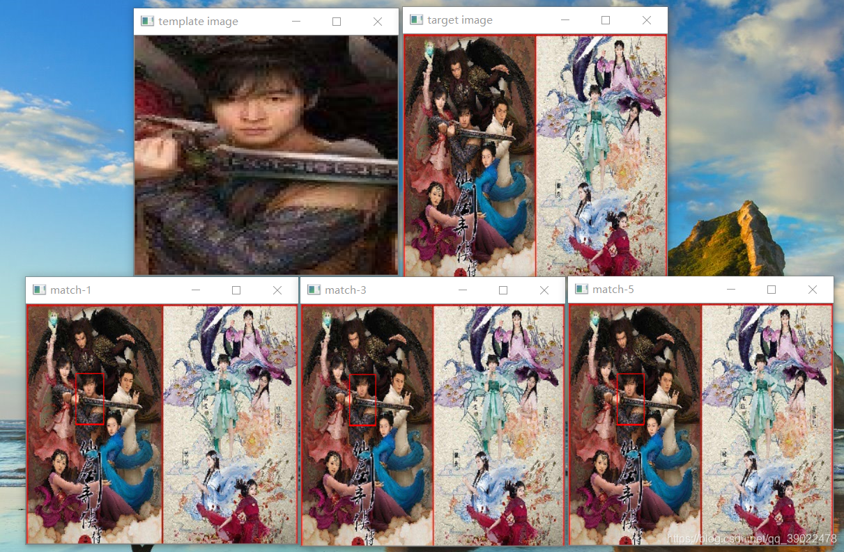
模板匹配在使用时需要注意模板图和输入图的比例关系，如果比例不同应当先调整再匹配。

注：本文是数字图像处理和深度之眼图像课程的学习笔记，由课程作业和ppt整理而来，仅用于学习交流。

OPENCV图像处理基础

OPENCV图像处理基础

1.图像处理基础

1.1 数字图像

1.1.1 数字图像概念：

1.1.2 数字图像起源：

1.1.3 常见成像方式：

1.1.4 数字图像的应用：

1.1.5 Opencv介绍：

1.2 图像属性

1.2.1 图像格式：

1.2.2 图像尺寸：

1.2.3 图像分辨率和通道：

1.2.4 图像直方图：

1.2.5 图像颜色空间：

1.3 本章代码实现

2.图像基本操作与opencv代码实现

2.1 Opencv中的绘图函数

2.2 图像的几何变换

2.3 图像滤波与增强

2.4 形态学操作

3.图像分割与代码实现

3.1 图像分割概念

3.2 固定阈值法

3.3 自动阈值法

3.4 边缘检测/提取

3.5 连通区域分析

3.6 区域生长算法

4.图像特征提取与代码实现

4.1 图像特征理解

4.2 形状特征

4.2.1 Hog特征提取

4.2.2 Harris角点检测

4.2.3 SIFT

4.3 纹理特征 LBP

4.4 模板匹配

猜你喜欢