数字图像处理python基础 （二）

python图像处理基础（二）

写在前面的话： 方便以后查文档，且这篇文章会随着学习一直更（因为还有opencv还没怎么学，目前是一些基本的操作）。都是跟着学习资料巩固的，只供学习使用。这一篇分为俩部分—— 边缘提取 与 形态学处理。 其实这部分内容太多了，我也只记录了部分方法的代码实现，还有很多需要在应用中体现。

第一部分—— 图像分割 (边缘提取)

阈值分割、边缘分割、基于区域的分割、Hough变换

阈值分割 二值化

from PIL import Image
import numpy as np
import matplotlib.pyplot as plt
%matplotlib inline

def thresholding(im, threshold=128):
    seg = np.zeros(im.shape)
    seg[im > threshold] = 255
    return seg

边缘分割
基本原理是检测图像中灰度变化较为显著的位置，即求图像在各个像素位置的梯度。

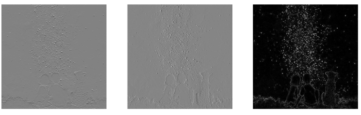
• sobel

im = array(Image.open('G:/photo/创意/1.jpg').convert('L'))

#Sobel derivative filters
""" 1代表y方向梯度，0代表x方向梯度 """
imy = zeros(im.shape)
filters.sobel(im,1,imy) #
imx = zeros(im.shape)
filters.sobel(im,0,imx)

magnitude = sqrt(imx**2+imy**2)

plt.figure(figsize=(18,12))
plt.gray()
plt.subplot(131)
plt.imshow(imx)

plt.axis('off')
plt.subplot(132)
plt.imshow(imy)

plt.axis('off')
plt.subplot(133)
plt.imshow(magnitude)
plt.axis('off')
plt.show()

基于梯度近似计算的边缘检测方法得到的边缘位置不精确，对图像噪声较为敏感。图像在物体边缘处的一阶导数会产生一个极值，因此二阶导数会存在一个过零点。过零点比极值点更容易确定。那么我们应该怎么样可靠的计算二阶导数？

1. 对图像进行平滑、再计算二阶导数
2. 先用Gaussian算子进行图像平滑，在用Laplace算子求解二阶导数：

• LoG (Laplacian of Gaussian)
  5×5离散LoG算子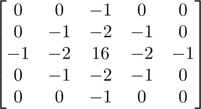
  

当标准差增大时所需卷积核的大小也相应增大。LoG算子可以用两个标准差不同的Gaussians算子卷积结果的差近似计算，也叫DoG(difference of Gaussians)算子。

def zero_cross(im):
    # 过零点检测（背景中的明亮噪声点）
    res = zeros(im.shape,dtype=float)
    m,n = im.shape

    for i in range(m-1):
        for j in range(n-1):
            if (im[i,j]*im[i+1,j]<0) or (im[i,j]*im[i,j+1]<0)  or (im[i,j]*im[i+1,j+1]<0) or (im[i,j+1]*im[i+1,j]<0):
                res[i,j]=1
    return res

def post_procesing(im,edge,threshold=0.2):
    # 用sobel算子计算一阶梯度
    imy = zeros(im.shape)
    filters.sobel(im,1,imy)
    imx = zeros(im.shape)
    filters.sobel(im,0,imx)
    magnitude = sqrt(imx**2+imy**2)

    # 去除一阶梯度角度的过零点
    edge_res = zeros(im.shape)
    edge_res[:] = edge
    edge_res[magnitude<threshold]=0

    return edge_res

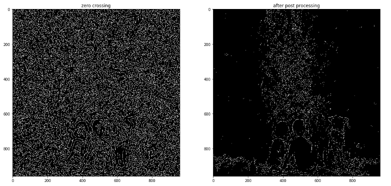
• 过零检测
  • 在获得LoG或DoG的结果后，利用过零检测就可以获得边缘的位置。
  • 利用一个2×2的滑动窗口
  • 如果某个方向的极性有变化就可以认为是过零点
  • 通常需要后处理：去掉一阶导数很小的位置

im = array(Image.open('G:/photo/创意/1.jpg').convert('L'))/255.0

im1 = ndimage.filters.gaussian_filter(im,4)
im2 = ndimage.filters.gaussian_filter(im,6)

imd = im2 - im1 # DoG
sd = ndimage.laplace(im1) # LoG

edge = zero_cross(sd)
edge_f = post_procesing(im,edge)

plt.figure(figsize=(18,12))
plt.subplot(121)
plt.imshow(sd)
plt.title(r'LoG,$\sigma=4$')
plt.subplot(122)
plt.imshow(imd)
plt.title(r'DoG,$\sigma_1=4,\sigma_2=6$')
plt.show()

plt.figure(figsize=(18,12))
plt.gray()
plt.subplot(121)
plt.imshow(edge)
plt.title('zero crossing')
plt.subplot(122)
plt.imshow(edge_f)
plt.title('after post processing')
plt.show()

顺便介绍几个常用的算子

• Roberts 算子
• Prewitt 算子
• Laplace 算子
• Kirsch 算子

具体可看 常见边界提取算子

基于区域的分割

分裂-归并分割算法

• 定义一个划分为区域的初始分割、一致性准则、金字塔数据结构。
• 如果在金字塔数据结构中的任意一个区域不是一致的，就将其分裂为4个子区域；如果具有相同的父节点的四个区域可以归并为单个一致性区域，则归并它们。如果没有区域可以分裂或归并，则转第3步。
• 如果任意两个邻接区域可以归并为一个一致性区域，则将它们归并。
• 如果必须删除小尺寸区域，则将小区域与其最相似的邻接区域归并。

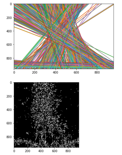
Hough变换

图像空间中共线的点在参数空间中对应的直线相交于同一点

• 使用Hough变换的曲线检测

1. 在参数a的范围内量化参数空间。参数空间的维数n与向量a的参数个数相等；
2. 创建一个n维的累计数组A(a)，其结构与参数空间的量化想匹配；所有元素初始化维0；
3. 在适当地阈值化后的梯度图像中，对每个图像点(x1,x2)，对应所有在第1步范围内的a，增大所有满足f(x,a)=0的累计单元A(a)；
4. 累计数组A(a) 中的局部极大值对应于出现在原始图像中的曲线f(x,a)=0 。

参数空间直线可以写为：
$s=xcos\theta+ysin\theta$

import cv2
new_path = 'G:/photo/innovation/1.jpg'
im = cv2.imread(new_path)

edges = cv2.Canny(im,5,100)
lines = cv2.HoughLines(edges,0.5,0.1,100)

x = np.array([0,im.shape[1]])
for line in lines:
    y = (line[0,0] - x*np.cos(line[0,1]))/np.sin(line[0,1])
    plt.plot(x,y)

plt.axis([0, im.shape[1], im.shape[0],0])

plt.figure()
plt.gray()
plt.imshow(edges)

plt.show()

Hough变换的特点：

• 可以检测图像中残缺的直线
• 对图像噪声不敏感
• 对其它共存的非直线结构不敏感
• 可以获得直线的解析方程
• 对于有先验知识的情况，可以有效地剔除不符合先验知识的直线
• 需要首先做二值化以及边缘检测等图像预处理工作，损失掉原始图像中的许多信息

第二部分—— 形态学处理

连通域处理、腐蚀与膨胀

连通域处理

在二值图像中，如果两个像素点相邻且值相同（同为0或同为1），那么就认为这两个像素点在一个相互连通的区域内。而同一个连通区域的所有像素点，都用同一个数值来进行标记，这个过程就叫连通区域标记

skimage.measure.label（image,connectivity=None)

• 参数中的image表示需要处理的二值图像，connectivity表示连接的模式，1代表4邻接，2代表8邻接。

• 输出一个标记数组（labels), 从0开始标记

from PIL import Image
import numpy as np
import matplotlib.pyplot as plt
from scipy.ndimage import measurements,morphology

im = np.array(Image.open('G:/photo/创意/1.jpg').convert('L'))
im_s = (im > 30)

此时 im_s 返回的是布尔值，也可直接放入函数，显示出每个连通域的像素个数，可以对其进行后续处理

labels, nbr_objects = measurements.label(im_s)
for i in range(1,nbr_objects+1):
    area = np.sum(labels == i)
    print('No.{}: {}'.format(i,area))
    if area < 100 or area >5000:
        labels[labels==i]=0 # 去除不符合条件的区域

腐蚀与膨胀、开运算与闭运算

膨胀 binary_dilation，可以将不同区域不同的显示出来

im = (im>128)
im_d = morphology.binary_dilation(im,np.ones((50,50)))

labels, nbr = measurements.label(im_d)
labels = labels * im

plt.gray()
plt.imshow(labels)
plt.show()

进行一次开运算 binary_opening ，看一下连通域像素的变化

• 第一个参数为图片，第二个为卷积核

im = np.array(Image.open('G:/photo/创意/1.jpg').convert('L'))
im = (im<128)

labels, nbr_objects = measurements.label(im)
print( "Number of objects:", nbr_objects)

# morphology - opening to separate objects better
im_open = morphology.binary_opening(im,np.ones((9,5)),iterations=2) 

labels_open, nbr_objects_open = measurements.label(im_open)
print( "Number of objects:", nbr_objects_open)