开篇
在NLP的前一篇文章,我希望关注的点就是我们文本的表示,说浅显一点就是词语的向量化,前面我们使用了one-hot编码,使用词袋模型,但是词袋模型几乎在现在的NLP任务中是不被使用的,只是作为一个入门的基础,我们是需要慢慢过渡到我们要使用的词向量去,当然在说词向量之前,我们还是要提一下一个比较重要的概念TF-IDF。
TF-IDF
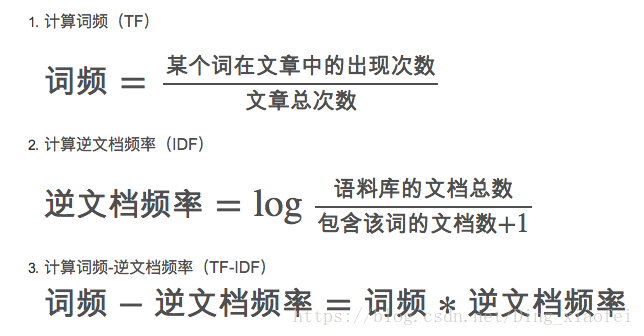
TF-IDF是Text Frequency – Inverse Document Frequency的缩写,很显然从字面意思上,TF-IDF是由两部分组成的,前半部分是词频,后半部分是逆文档频率。TF-IDF是衡量单词重要性的一种指标。
任务
关于任务的介绍可以参照之前的博客词袋模型,里面有详细的解说,这边就明确一下我们的基本任务吧,输入是一条短信的文本,输出是是否是垃圾短信的分类类别。在本文的最后我会放上完整的代码。为了避免数据放置位置的错误,我将数据集的下载和放置直接写在了代码里面,也就是说,代码是可以直接跑的,只要你的环境是没有问题的。
代码
日常的预处理
texts = [x[1] for x in text_data]
target = [x[0] for x in text_data]

# Relabel 'spam' as 1, 'ham' as 0
target = [1. if x=='spam' else 0. for x in target]

# Normalize text
# Lower case
texts = [x.lower() for x in texts]

# Remove punctuation
texts = [''.join(c for c in x if c not in string.punctuation) for x in texts]

# Remove numbers
texts = [''.join(c for c in x if c not in '0123456789') for x in texts]

# Trim extra whitespace
texts = [' '.join(x.split()) for x in texts]
下面就是我们的核心部分,TF-IDF的处理,我们的TensorFlow没有直接处理TF-IDF的函数,所以这边我们调用sklearn这个机器学习库来生成我们每一个单词的tf-idf值,请看代码:
def tokenizer(text):
    words = nltk.word_tokenize(text)
    return words

# Create TF-IDF of texts
tfidf = TfidfVectorizer(tokenizer=tokenizer, stop_words='english', max_features=max_features)
sparse_tfidf_texts = tfidf.fit_transform(texts)
最上面的那个函数是一个分词函数,使用的是NLTK这个NLP的python库,效果其实就是这样的
In [1]: import nltk

In [2]: a = "my name is tensorflow"

In [3]: a = nltk.word_tokenize(a)

In [4]: a
Out[4]: ['my', 'name', 'is', 'tensorflow']
先解释一下TfidfVectorizer函数里面的几个参数,第一个是分词函数,第二个它会默认去掉一些停用词,第三个是取频率靠前多少的那些词。这里我们取的是频率
下面有一个简单的示例,给你展示一下,这个函数到底是在作用什么?
In [1]: from sklearn.feature_extraction.text import TfidfVectorizer

In [2]: corpus = [
   ...:     'This is the first document.',
   ...:     'This is the second second document.',
   ...:     'And the third one.',
   ...:     'Is this the first document?',
   ...: ]

In [3]: vectorizer = TfidfVectorizer()

In [5]: vectorizer.fit_transform(corpus)
Out[5]:
<4x9 sparse matrix of type '<class 'numpy.float64'>'
    with 19 stored elements in Compressed Sparse Row format>
其实重要的就这几步,这里是已经生成了tf-idf值了。
In [6]: a = vectorizer.fit_transform(corpus)

In [7]: print(a[0])
  (0, 8)    0.438776742859
  (0, 3)    0.438776742859
  (0, 6)    0.358728738248
  (0, 2)    0.541976569726
  (0, 1)    0.438776742859
这里我们存储的是典型的系数矩阵,前面的一个元组代表的是第0句,在词典里面的第8位的词,那么词典是什么样的呢?
In [8]: vectorizer.get_feature_names()
Out[8]: ['and', 'document', 'first', 'is', 'one', 'second', 'the', 'third', 'this']
注意上面我们任务代码中是有一个参数的max_features,这代表的是我们词典的长度,我们取词频前max_features的词作为我们的词典,那么我们每句产生的词语权值也就是max_features长度的啦。因为我们要用它来代表我们的句子,作为我们的一种句向量。下面让我们看看这里的句向量是什么吧?

In [9]: a.toarray()
Out[9]:
array([[ 0.        ,  0.43877674,  0.54197657,  0.43877674,  0.        ,
         0.        ,  0.35872874,  0.        ,  0.43877674],
       [ 0.        ,  0.27230147,  0.        ,  0.27230147,  0.        ,
         0.85322574,  0.22262429,  0.        ,  0.27230147],
       [ 0.55280532,  0.        ,  0.        ,  0.        ,  0.55280532,
         0.        ,  0.28847675,  0.55280532,  0.        ],
       [ 0.        ,  0.43877674,  0.54197657,  0.43877674,  0.        ,
         0.        ,  0.35872874,  0.        ,  0.43877674]])
每一句的长度都是词典的长度,句子出现单词对应的词典位置上都是我们的tf-idf的值,这样大概大家就应该知道上面那些元组代表的就是一种索引,这里也是为了节约存储空间,所以存成索引加值的方式。而我们任务中怎么把这种方式转换成正常的句子向量呢?
In [11]: print(a[0])
  (0, 8)    0.438776742859
  (0, 3)    0.438776742859
  (0, 6)    0.358728738248
  (0, 2)    0.541976569726
  (0, 1)    0.438776742859

In [12]: a[0].todense()
Out[12]:
matrix([[ 0.        ,  0.43877674,  0.54197657,  0.43877674,  0.        ,
          0.        ,  0.35872874,  0.        ,  0.43877674]])

In [13]: a.todense()
Out[13]:
matrix([[ 0.        ,  0.43877674,  0.54197657,  0.43877674,  0.        ,
          0.        ,  0.35872874,  0.        ,  0.43877674],
        [ 0.        ,  0.27230147,  0.        ,  0.27230147,  0.        ,
          0.85322574,  0.22262429,  0.        ,  0.27230147],
        [ 0.55280532,  0.        ,  0.        ,  0.        ,  0.55280532,
          0.        ,  0.28847675,  0.55280532,  0.        ],
        [ 0.        ,  0.43877674,  0.54197657,  0.43877674,  0.        ,
          0.        ,  0.35872874,  0.        ,  0.43877674]])

In [14]: a[0].toarray()
Out[14]:
array([[ 0.        ,  0.43877674,  0.54197657,  0.43877674,  0.        ,
         0.        ,  0.35872874,  0.        ,  0.43877674]])
这里的是toarray()和todense()效果是一样的,但事实上它们还是有所区别的,这边就姑且当它们一样吧,留个坑,以后我再来填。我想讲到这里,大家应该知道tf-idf怎么操作了。到这里我们今天的任务就基本完成大半啦。
下面继续回到我们的任务代码里面
首先是数据集的划分
# Split up data set into train/test
train_indices = np.random.choice(sparse_tfidf_texts.shape[0], round(0.8*sparse_tfidf_texts.shape[0]), replace=False)
test_indices = np.array(list(set(range(sparse_tfidf_texts.shape[0])) - set(train_indices)))
texts_train = sparse_tfidf_texts[train_indices]
texts_test = sparse_tfidf_texts[test_indices]
target_train = np.array([x for ix, x in enumerate(target) if ix in train_indices])
target_test = np.array([x for ix, x in enumerate(target) if ix in test_indices])这边稍微插一句,enumerate是为了解决python里面for循环没有下标的问题的。
下面就是我们模型的设定和模型预测
# Create variables for logistic regression
A = tf.Variable(tf.random_normal(shape=[max_features,1]))
b = tf.Variable(tf.random_normal(shape=[1,1]))

# Initialize placeholders
x_data = tf.placeholder(shape=[None, max_features], dtype=tf.float32)
y_target = tf.placeholder(shape=[None, 1], dtype=tf.float32)

# Declare logistic model (sigmoid in loss function)
model_output = tf.add(tf.matmul(x_data, A), b)

# Declare loss function (Cross Entropy loss)
loss = tf.reduce_mean(tf.nn.sigmoid_cross_entropy_with_logits(logits=model_output, labels=y_target))

# Actual Prediction
prediction = tf.round(tf.sigmoid(model_output))
predictions_correct = tf.cast(tf.equal(prediction, y_target), tf.float32)
accuracy = tf.reduce_mean(predictions_correct)
tf.round的作用如下
舍入最接近的整数
# ‘a’ is [0.9, 2.5, 2.3, -4.4]
tf.round(a) ==> [ 1.0, 3.0, 2.0, -4.0 ]
讲一讲这边模型的维度问题,我们使用sklearn里面的tfidf工具训练出来了频率靠前的1000个词的tf-idf值,我们用这1000个维度来表示我们每一句的向量,当我们句子出现了某个词,那么某个词的那一位上就有它的tf-idf值,如果没有出现某个词,那么那个词的那一位我们就用0来表示,那么我们输入的x就是一个长度为1000的句向量。
关于训练的一些问题再讲一下
for i in range(10000):
    rand_index = np.random.choice(texts_train.shape[0], size=batch_size)
    rand_x = texts_train[rand_index].todense()
    rand_y = np.transpose([target_train[rand_index]])
    sess.run(train_step, feed_dict={x_data: rand_x, y_target: rand_y})
这边的np.transpose是转置,这里的训练就是一次拿个batch_size的数据来训练,训练个10000次啦。
最后附上我们的完整代码以供大家参考
import tensorflow as tf
import matplotlib.pyplot as plt
import csv
import numpy as np
import os
import string
import requests
import io
import nltk
from zipfile import ZipFile
from sklearn.feature_extraction.text import TfidfVectorizer
from tensorflow.python.framework import ops
ops.reset_default_graph()

# Start a graph session
sess = tf.Session()

batch_size = 200
max_features = 1000


# Check if data was downloaded, otherwise download it and save for future use
save_file_name = 'temp_spam_data.csv'
if os.path.isfile(save_file_name):
    text_data = []
    with open(save_file_name, 'r') as temp_output_file:
        reader = csv.reader(temp_output_file)
        for row in reader:
            text_data.append(row)
else:
    zip_url = 'http://archive.ics.uci.edu/ml/machine-learning-databases/00228/smsspamcollection.zip'
    r = requests.get(zip_url)
    z = ZipFile(io.BytesIO(r.content))
    file = z.read('SMSSpamCollection')
    # Format Data
    text_data = file.decode()
    text_data = text_data.encode('ascii',errors='ignore')
    text_data = text_data.decode().split('\n')
    text_data = [x.split('\t') for x in text_data if len(x)>=1]

    # And write to csv
    with open(save_file_name, 'w') as temp_output_file:
        writer = csv.writer(temp_output_file)
        writer.writerows(text_data)


texts = [x[1] for x in text_data]
target = [x[0] for x in text_data]

# Relabel 'spam' as 1, 'ham' as 0
target = [1. if x=='spam' else 0. for x in target]

# Normalize text
# Lower case
texts = [x.lower() for x in texts]

# Remove punctuation
texts = [''.join(c for c in x if c not in string.punctuation) for x in texts]

# Remove numbers
texts = [''.join(c for c in x if c not in '0123456789') for x in texts]

# Trim extra whitespace
texts = [' '.join(x.split()) for x in texts]

# Define tokenizer
def tokenizer(text):
    words = nltk.word_tokenize(text)
    return words

# Create TF-IDF of texts
tfidf = TfidfVectorizer(tokenizer=tokenizer, stop_words='english', max_features=max_features)
sparse_tfidf_texts = tfidf.fit_transform(texts)

# Split up data set into train/test
train_indices = np.random.choice(sparse_tfidf_texts.shape[0], round(0.8*sparse_tfidf_texts.shape[0]), replace=False)
test_indices = np.array(list(set(range(sparse_tfidf_texts.shape[0])) - set(train_indices)))
texts_train = sparse_tfidf_texts[train_indices]
texts_test = sparse_tfidf_texts[test_indices]
target_train = np.array([x for ix, x in enumerate(target) if ix in train_indices])
target_test = np.array([x for ix, x in enumerate(target) if ix in test_indices])

# Create variables for logistic regression
A = tf.Variable(tf.random_normal(shape=[max_features,1]))
b = tf.Variable(tf.random_normal(shape=[1,1]))

# Initialize placeholders
x_data = tf.placeholder(shape=[None, max_features], dtype=tf.float32)
y_target = tf.placeholder(shape=[None, 1], dtype=tf.float32)

# Declare logistic model (sigmoid in loss function)
model_output = tf.add(tf.matmul(x_data, A), b)

# Declare loss function (Cross Entropy loss)
loss = tf.reduce_mean(tf.nn.sigmoid_cross_entropy_with_logits(logits=model_output, labels=y_target))

# Actual Prediction
prediction = tf.round(tf.sigmoid(model_output))
#舍入最接近的整数
predictions_correct = tf.cast(tf.equal(prediction, y_target), tf.float32)
accuracy = tf.reduce_mean(predictions_correct)

# Declare optimizer
my_opt = tf.train.GradientDescentOptimizer(0.0025)
train_step = my_opt.minimize(loss)

# Intitialize Variables
init = tf.global_variables_initializer()
sess.run(init)

# Start Logistic Regression
train_loss = []
test_loss = []
train_acc = []
test_acc = []
i_data = []
for i in range(10000):
    rand_index = np.random.choice(texts_train.shape[0], size=batch_size)
    rand_x = texts_train[rand_index].todense()
    rand_y = np.transpose([target_train[rand_index]])
    sess.run(train_step, feed_dict={x_data: rand_x, y_target: rand_y})

    # Only record loss and accuracy every 100 generations
    if (i+1)%100==0:
        i_data.append(i+1)
        train_loss_temp = sess.run(loss, feed_dict={x_data: rand_x, y_target: rand_y})
        train_loss.append(train_loss_temp)

        test_loss_temp = sess.run(loss, feed_dict={x_data: texts_test.todense(), y_target: np.transpose([target_test])})
        test_loss.append(test_loss_temp)

        train_acc_temp = sess.run(accuracy, feed_dict={x_data: rand_x, y_target: rand_y})
        train_acc.append(train_acc_temp)

        test_acc_temp = sess.run(accuracy, feed_dict={x_data: texts_test.todense(), y_target: np.transpose([target_test])})
        test_acc.append(test_acc_temp)
    if (i+1)%500==0:
        acc_and_loss = [i+1, train_loss_temp, test_loss_temp, train_acc_temp, test_acc_temp]
        acc_and_loss = [np.round(x,2) for x in acc_and_loss]
        print('Generation # {}. Train Loss (Test Loss): {:.2f} ({:.2f}). Train Acc (Test Acc): {:.2f} ({:.2f})'.format(*acc_and_loss))


# Plot loss over time
plt.plot(i_data, train_loss, 'k-', label='Train Loss')
plt.plot(i_data, test_loss, 'r--', label='Test Loss', linewidth=4)
plt.title('Cross Entropy Loss per Generation')
plt.xlabel('Generation')
plt.ylabel('Cross Entropy Loss')
plt.legend(loc='upper right')
plt.show()

# Plot train and test accuracy
plt.plot(i_data, train_acc, 'k-', label='Train Set Accuracy')
plt.plot(i_data, test_acc, 'r--', label='Test Set Accuracy', linewidth=4)
plt.title('Train and Test Accuracy')
plt.xlabel('Generation')
plt.ylabel('Accuracy')
plt.legend(loc='lower right')
plt.show()