1.Comprehensive narrative(综述部分)
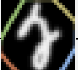
(1)CNN网络有一个显著的缺点就是对于识别数据缺少一定的空间转换能力,比如你正着,斜着,倒着看你自己的水杯都可以知道这是你的水杯而CNN却不一定行。如下图:
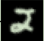
你一定知道这全部是数字2

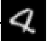
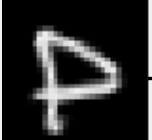
你一定知道这全部是数字4 !

基于上述的原因,本文作者给出了STN(空间转换网络)针对解决CNN缺少的空间转换能力
2.Abstract
本文摘要主要讲述了CNN缺少使输入的数据保持空间不变,作者给出了新的可学习的模块-空间转换器。这个模块可以直接插入已经存在的卷积结构并提供给该网络结构进行空间转换的能力,此外,该模块不需要额外的监督训练和修改优化。原文如下:
Convolutional Neural Networks define an exceptionally powerful class of models,but are still limited by the lack of ability to be spatially invariant to the input data in a computationally and parameter efficient manner. In this work we introduce a new learnable module, the Spatial Transformer, which explicitly allows the spatial manipulation of data within the network. This differentiable module can be inserted into existing convolutional architectures, giving neural networks the ability to actively spatially transform feature maps, conditional on the feature map itself, without any extra training supervision or modification to the optimisation process. We show that the use of spatial transformers results in models which learn invariance to translation, scale, rotation and more generic warping, resulting in state-of-the-art performance on several benchmarks, and for a number of classes of transformations.
3.Introduction
(1)虽然池化层提供了一些空间变换能力,但是由于池化感受野窗口大小一般只有2×2大小的窗口只会对深层的卷积和特征有作用。
(2)空间转换可以在整个特征图上进行进行缩放,修剪,旋转和一些非刚性变换。
(3)空间转换换可以对图像进行高相关性选取(类似Attention)和规范化(后文有涉及)。
(4)空间转换可以组装进CNN中使很多任务受益:1.图像分类 2.共同定位 3.空间Attention
4.Spatial transformers (Essential Point)
在空间转换网络中主要分以下3个部分(1)Localisation Network
(2)Parameterized Sampling Grid (3)Differentable Image Sampling
(1)localisation network 主要完成回归仿射转换矩阵theta(theta中包括旋转,平移,缩放等参数),其中该网络即可以是全连接网络也可以是卷积网络
(2)Parameterized Sampling Grid 主要生成和图片像素点一致的采样网格,并与theta矩阵相乘逐渐学习到完全对应倾斜识别物
(1)Differentable Image Sampling 主要是通过获取采样点对应的原图像像素点形成 V 特征图完成对 V 特征图的输出

(1)Localisation Network
Localisation Network 这个部分对应着是回归预测θ仿射变换系数,其中θ为一个6维参数用于对特征图进行转换。
The localisation network takes the input feature map with width W, height H and C channels and outputs θ, the parameters of the transformation to be applied to the feature map: θ = f loc (U). The size of θ can vary depending on the transformation type that is parameterised, e.g. for an affine transformation θ is 6-dimensional as in (1).
#读取图片
input_img = np.concatenate([img1, img2, img3, img4], axis=0)

B, H, W, C = input_img.shape

print("Input Img Shape: {}".format(input_img.shape))

# identity transform
theta = np.array([[1., 0, 0], [0, 1., 0]])

x = tf.placeholder(tf.float32, [None, H, W, C])

with tf.variable_scope('spatial_transformer'):
    theta = theta.astype('float32')
    theta = theta.flatten()

    # 定义可优化参数变形θ的权重和偏置
    loc_in = H*W*C
    loc_out = 6
    W_loc = tf.Variable(tf.zeros([loc_in, loc_out]), name='W_loc')
    b_loc = tf.Variable(initial_value=theta, name='b_loc')

    # fc_loc就是文中所提及的可训练变形参数θ,B为样本的batch_szie
    # θ的shape=[B,H*W*C] * [H*W*C,6]+[6]=[B,6]

    fc_loc = tf.matmul(tf.zeros([B, loc_in]), W_loc) + b_loc
接下来传入image/features map 以及theta参数进入Spatial Transformer
def spatial_transformer_network(input_fmap, theta, out_dims=None, **kwargs):

    # grab input dimensions
    B = tf.shape(input_fmap)[0]
    H = tf.shape(input_fmap)[1]
    W = tf.shape(input_fmap)[2]

    # reshape theta to (B, 2, 3)
    theta = tf.reshape(theta, [B, 2, 3])

    # generate grids of same size or upsample/downsample if specified
    # 如果有降采样或重采样的要求传入 out_dims 一般是elese语句:
    if out_dims:
        out_H = out_dims[0]
        out_W = out_dims[1]

        #进入Parameterised Sampling Grid
        batch_grids = affine_grid_generator(out_H, out_W, theta)
    else:
        batch_grids = affine_grid_generator(H, W, theta)

    x_s = batch_grids[:, 0, :, :]
    y_s = batch_grids[:, 1, :, :]

    # sample input with grid to get output
    out_fmap = bilinear_sampler(input_fmap, x_s, y_s)

    return out_fmap
(2)Parameterised Sampling Grid
对于仿射变换,如果直接由仿射变换系数θ对输入(x,y)求解得到输出坐标点( , )是非整数的,因此需要对考虑逆向仿射变换。所谓逆向仿射变换就是首先根据仿射变换输出的大小,生成输出的坐标网格点(下面代码中有涉及).例如V的大小为10×1010×10时,我们便可以得到一个10×1010×10大小的坐标位置点矩阵,接下来就是要对该坐标位置点进行仿射变换,仿射变换公式及示意图如下:

其中
为2D仿射变换矩阵,
代表的是输出features maps的坐标点也可以说是像素点,
代表的是输入feature map的对应坐标点(像素点)。
其中
=
这样来看
×
=
可以看做是
× 仿射变换s + x的平移量
= 新的坐标点
这个方式的目标是创建一个区域,将歪曲原图中的对应像素点填补到创建的区域当中
def affine_grid_generator(height, width, theta):

    num_batch = tf.shape(theta)[0]

    #创建一个规范化2D网格
    #将 -1.0到1.0分为 width 份
    x = tf.linspace(-1.0, 1.0, width)
     #将 -1.0到1.0分为 height 份
    y = tf.linspace(-1.0, 1.0, height)
    #将x轴方向扩大为width份x
    eg:[[0,1], [0,1]]

    #将y轴方向扩大为height份y
    eg:[[0,0],[1,1]]
    x_t, y_t = tf.meshgrid(x, y)

   #reshape为一维向量 shape=[width*hight]
   eg:[0,1,0,1]
    x_t_flat = tf.reshape(x_t, [-1])
    eg:[0,0,1,1]
    y_t_flat = tf.reshape(y_t, [-1])

   #初始化width*hight个1 shape=[width*hight]
    ones = tf.ones_like(x_t_flat)
   #将三个一维向量组成二维向量 shape=[3,hight*width]
    sampling_grid = tf.stack([x_t_flat, y_t_flat, ones])

    # repeat grid num_batch times
    #扩充维度为[1,3,width*height]
    sampling_grid = tf.expand_dims(sampling_grid, axis=0)
   #改变维度为[num_batch,3,width*height]
    sampling_grid = tf.tile(sampling_grid, tf.stack([num_batch, 1, 1]))

    # cast to float32 (required for matmul)
    theta = tf.cast(theta, 'float32')
    sampling_grid = tf.cast(sampling_grid, 'float32')

    # 对规范化网格进行transformer得出inputmap的真实x的代值,y的代值对应下面的word1
    #当所有的代值 × 图片的像素H,W全部转化为各自的x,y,如下图:
    #[num_batch,2,3]×[num_batch,3,width*height]=[num_batch,2,width*height]

    batch_grids = tf.matmul(theta, sampling_grid)


    # reshape to (num_batch, H, W, 2)
    batch_grids = tf.reshape(batch_grids, [num_batch, 2, height, width])

    return batch_grids
word1:其中
=
这样来看
×
=
可以看做是
× 仿射变换s + x的平移量
= 新的坐标点
。第一行为x,第二行为y

3.Differentable Image Sampling
这个部分随着输入的特征图U,通过规范化网格中的采样点输出特征图V
#x,y就是上一步中的坐标点,第一行取出的x,第二行取出的y
    x_s = batch_grids[:, 0, :, :]
    y_s = batch_grids[:, 1, :, :]
    #调用下列函数
    out_fmap = bilinear_sampler(input_fmap, x_s, y_s)

def bilinear_sampler(img, x, y):
#原始图像的H
    H = tf.shape(img)[1]
    #原始图像的W
    W = tf.shape(img)[2]
    #因为取图像中的值是从0开始,所以全部-1
    max_y = tf.cast(H - 1, 'int32')
    max_x = tf.cast(W - 1, 'int32')
    zero = tf.zeros([], dtype='int32')

    # rescale x and y to [0, W-1/H-1]
    x = tf.cast(x, 'float32')
    y = tf.cast(y, 'float32')

    #用规范化网格中的代值[-1,1]×真实图像tensor中得出每个坐标的真实值
    x = 0.5 * ((x + 1.0) * tf.cast(max_x-1, 'float32'))
    y = 0.5 * ((y + 1.0) * tf.cast(max_y-1, 'float32'))

    # grab 4 nearest corner points for each (x_i, y_i)
    x0 = tf.cast(tf.floor(x), 'int32')
    x1 = x0 + 1
    y0 = tf.cast(tf.floor(y), 'int32')
    y1 = y0 + 1

    # 返回值取值出现越界现象,将所有x,y规范到【0,width/height-1】之间
    x0 = tf.clip_by_value(x0, zero, max_x)
    x1 = tf.clip_by_value(x1, zero, max_x)
    y0 = tf.clip_by_value(y0, zero, max_y)
    y1 = tf.clip_by_value(y1, zero, max_y)

    # 取对应坐标中的真实图像tensor的value
    Ia = get_pixel_value(img, x0, y0)
    Ib = get_pixel_value(img, x0, y1)
    Ic = get_pixel_value(img, x1, y0)
    Id = get_pixel_value(img, x1, y1)

    # recast as float for delta calculation
    x0 = tf.cast(x0, 'float32')
    x1 = tf.cast(x1, 'float32')
    y0 = tf.cast(y0, 'float32')
    y1 = tf.cast(y1, 'float32')

    # calculate deltas
    wa = (x1-x) * (y1-y)
    wb = (x1-x) * (y-y0)
    wc = (x-x0) * (y1-y)
    wd = (x-x0) * (y-y0)

    # add dimension for addition
    wa = tf.expand_dims(wa, axis=3)
    wb = tf.expand_dims(wb, axis=3)
    wc = tf.expand_dims(wc, axis=3)
    wd = tf.expand_dims(wd, axis=3)

    #生成V features map
    out = tf.add_n([wa*Ia, wb*Ib, wc*Ic, wd*Id])

    return out
然后论文给出了一些双线性插值法,当然也可以使用其他的采样方法,然而为了让梯度可以反向传播,使用的方法必须要可以对其参数进行求导。通过插值,我们可以改变最终输出V的大小,从而完成整个transformer。

至此,整个前向传播就完成了。与以往的网络稍微不同的就是STN中有一个采样(插值)的过程,这个采样需要依靠一个特定的网格作为引导。但是细想,我们常用的池化也是一种采样(插值)方式,只不过使用的网格有点特殊而已。
既然存在网络,需要训练,那么就必须得考虑损失的反向传播了。对于自己定义的sampler,这里的反向传播公式需要推导。 其中,输出对采样器的求导公式为:

4.Spatial Transformer Networks
这就是作者对空间转换网络的综述,第一段说空间转换网络的优点,速度快,巴拉巴拉的然后作者说H,W不能随便瞎玩,如果取的值小于了图片本身的H,W可能会导致混叠,之后告诉你可以使用多个空间转换网络,在网络的深处允许对越来越抽象的表示进行转换,同时也为本地化网络提供了潜在的更丰富的信息表示,以便根据预测的转换参数进行转换。
最后给出结果,提升了识别的准确率

