Graphics pipeline basics (2)
Article directory
foreword
In the previous article, we shared the general process of OpenGL, and then we will continue to share the next process - frame buffer operation. It is also our last stage.
1. Frame buffer operation
The framebuffer is the last stage of the Opengl graphics pipeline. This cache can represent the visible content of the screen. and other memory areas for storing per-pixel values except color. The framebuffer stores state including where data generated by the fragment shader should be written. Data format and other information. The state is kept in the framebuffer object. Pixel execution state is also considered part of the framebuffer, but is not stored per framebuffer object.
2. Frame buffer operation process
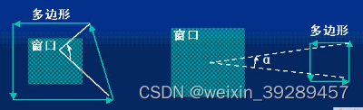
1. Cropping test
After the fragment shader generates output, the fragment will go through some steps before writing to the window, such as judging whether it belongs to the window, we can turn on or off these steps in the application. The first is the cropping test, that is, the fragment is tested according to the rectangle we defined, if the fragment is within the holding, it will be further processed, and if it is outside the rectangle, it will be discarded.
About cutting mainly introduces the following cutting methods:
1-1. Point clipping
The condition of point P in the window satisfies the following inequalities
Xmin <= x <= Xmax and Ymin <= y <= Ymax
otherwise it is outside the window
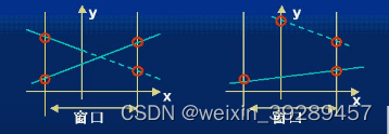
1-2. Straight line cutting
The relationship between straight lines and windows usually has the following three situations
: 1. The straight lines are all inside the window
; 2. The straight lines are all
outside the window;
Inside the window
1. When the two endpoints of a straight line are all inside the window, the straight line is entirely inside the window.
2. When the two endpoints of a straight line are inside the window and the other is outside the window, the part of the straight line is inside the window. Partially outside the window
3. When the two endpoints of a straight line are all outside the window, the straight line may be outside the entire window or partly inside the window and partly outside the window.
1. Cohen-Sutherland straight line clipping algorithm
Background: This is the earliest and most popular line clipping algorithm. The algorithm speeds up the line segment clipping algorithm by reducing the number of calculated intersection points through the initial test.
Principle: The end point of each line segment is assigned a four-digit binary code, which is called the area code. Used to identify the position of the endpoint relative to the clipping matrix boundaries. The area is set by the boundary as shown below.
The relationship between the clipping boundary of the area code is: up, down, right, left,
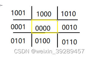
when any bit of X, X, X, X is assigned a value of 1, it means that the end point falls outside the corresponding boundary, otherwise the bit is 0, If the endpoint is in the clipping rectangle, the area code is 0, 0, 0, 0. If the endpoint falls in the lower left corner of the rectangle, the area code is 0, 1, 0, 1.
Once the area codes of all line segment endpoints are given, it can be Quickly judge which line is completely inside the clipping window and which line is completely outside the window, so the following rules are obtained:
1. If the codes of both endpoints are 0, 0, 0, 0, it means that the line is inside the
window2 .If the coding phase of the two endpoints is not 0,0,0,0, it means that the line is outside the window.
3. If the coding of the two endpoints is not all 0,0,0,0, but the phase AND is 0,0 , 0, 0 means that part of the line is visible, and the intersection point with the window needs to be calculated to determine which part is visible.
The key to the Sohen_Sutherland algorithm is to always determine an endpoint outside the window first, so that the line segment between this endpoint and the intersection point with the edge of the window must be invisible, so it can be discarded, and then use the same method to process the rest.
Its extended algorithm includes: take the midpoint judgment method, and cut the straight line with this.
Summary: The advantage of this algorithm is that it is simple and easy to implement. It can be simply described as deleting the part of the line outside the window, and proceeding in the order of up, down, left, and right. After processing, the remaining part is visible.
Finding the intersection point is very important in this algorithm, which determines the speed of the algorithm. The midpoint intersection method is very suitable for hardware. It can replace multiplication and division with left and right displacement, which greatly speeds up the speed.
2. Cyrus_Beck straight line clipping algorithm
Dot product of vectors
Let the two vectors be P and Q respectively, then their dot product is P . Q = |P||Q|cos#
If P . Q > 0, then the included angle# <90If
P . Q = 0, then its included angle # = 90
If P . Q < 0, then its included angle # >90 The
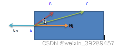
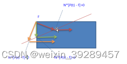
basic idea of the Cyrus-Beck algorithm is to use the concept of normal vector to determine whether a point of a line segment is inside the window or on the window boundary superior. For any convex polygon, the internal normal vector at any point on its boundary can be expressed by the vector dot product of line and surface: Nj . (B - A ) >= 0, a is a point on the polygon boundary, b is another point on the polygon boundary a little. The angle between Nj and any other vector from a to b must be no greater than 90
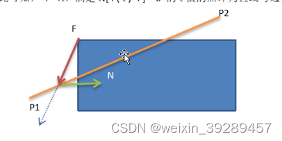
If f is a point on the boundary of the convex polygon, and N is the internal normal vector of the boundary of the convex area at point f, then for a point P(t) on the line segment P1, P2, the following formula is satisfied: 1. If N*[P(
t ) - f] < 0, it means that P(t) - f points to the outside of the region
2. If N*[P(t) - f] = 0, it means that P(t) - f coincides with the boundary containing f and perpendicular to the normal vector N.
3. If N*[P(t) - f] > 0, it means that P(t) - f points to the interior of the region.
It can be seen from this that the point where P(t) satisfies the t value of N[ P( t ) -f ] = 0 is the intersection point of the line and the boundary. In the Cyrus-Beck algorithm, the judgment of the
visibility of the line segment is as follows:
Set the internal normal vector Clicking on the vector connecting a point on the line segment to a point on the boundary is: N*[P(t) - f]
Set the line segment P1, P2 parameter equation: P(t) = P1 + (P2 - P1)t
combined to get: N* [P1 + (P2 - P1) t - f]
The condition that the point on the line segment is on the boundary: N*[P1 + (P2 - P1) t - f] = 0
Let D = P2 - P1, w= P1 - f It can be obtained that
t = - W . N/ D . N
If D . N = 0, then either vertical N, or P2 = P1
The relationship between point P1 and the window can be described as follows:
If w . n < 0, it means that point P is located in the window If
w . n = 0 , it means that the point P is located on the edge of the window
If w . n > 0 , it means that the point P is located in the window
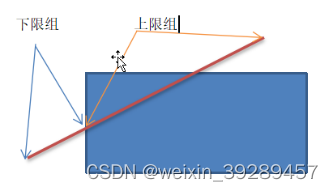
For the selection of t value: firstly, 0 <= t <= 1. Second, for a convex polygon, each line segment has at most two intersection points with it, that is, there are two corresponding t values, so we can calculate T The values are divided into two groups, one group is the upper limit group, which is distributed on the side of the starting point of the line segment, and the other group is the lower limit group, which is distributed on the side of the line segment end point, so as long as the maximum value in the lower limit group and the minimum value of the upper limit group are found The value can determine the line segment.
The basis of grouping:
if w . n < 0 , the calculated value belongs to the lower limit group.
If w . n > 0 , the calculated value belongs to the upper limit group
. With these, the entire algorithm is established
Cyrus -Beck algorithm summary
This algorithm is more widely used than the Cohen-Sutherland algorithm. It can be applied to any convex polygon, but it is invalid for concave polygons. The following is the method for determining convex polygons. For concave polygons we can also convert them into convex polygons by polygon cutting.
Judgment of convex polygon
Cross product method
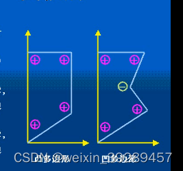
1. If each cross product is all zero, then the sides of the polygon are collinear.
2. If part of each cross product is positive and part is negative, the polygon is a concave polygon
. 3. If all cross products are all If it is greater than zero or equal to zero, the polygon is a convex polygon. At this time, along the positive direction of the edge, the inner normal vector points to its left side. 4.
If all cross products are less than zero or equal to zero, the polygon is a convex polygon. At this time, along the edge The positive direction of , the inner normal vector points to its right (the cross product follows the left-hand rule)
1-3. Polygon clipping
Polygon clipping can be decomposed into line segments one by one. The clipping of a polygon by a window can produce one or more edges if its closure is considered
1. Sutherland-Hodgeman polygon clipping algorithm
Polygon clipping is achieved by clipping a single edge or face. That is, in the algorithm, each side of the clipping window will successively perform clipping on the original polygon and the polygon generated by each clipping.
Each output of the clipping algorithm (including intermediate results) is a polygon vertex table, and all vertices are On the visible side of the corresponding window clipping edge or face. Since each edge of the polygon needs to be compared with the clipped edge or face separately, only the possible positional relationship between a single edge and a single clipped edge or face needs to be discussed. Assuming that S and P are two adjacent vertices of a polygon, and S is the starting point of the edge, and P is the end point of the edge, there are only 4 possible relationships between the edge SP and the clipping edge or face.
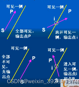
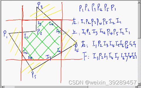
It can be seen from the above that after comparing the edge of the polygon with the clipped edge or face each time, one or two vertices are output, and there may be no output points. If the SP side is completely visible, then output point P, and do not need to output point S. Because vertices are processed sequentially. S is output as the end point of the previous side, if SP is completely invisible, no output point. If the SP edge is partially visible, the SP edge may enter or leave the visible side of the clipping edge or face. If the SP edge enters the visible side of the clipped edge or face, two points are output, one is the intersection of SP and the clipped edge or face, and the other is the P point.
For the first vertex of the polygon, it is only necessary to judge its visibility. If it is visible, output it and use it as the starting point S, otherwise there is no output point. But it is still necessary to save the S point for subsequent processing.
For the last edge PnP1, its processing method is: mark the first vertex as F, so that the last edge is PnF, which can be treated the same as other edges.
Summary of polygon clipping algorithm
Applying this algorithm to convex polygons can get correct results. But clipping for concave polygons will show an extra line as shown. This happens when the clipped polygon has two or more separate parts. Since there is only one output vertex table, the last vertex in the table is always connected to the first vertex.
There are many ways to solve this problem.
1. Divide the concave polygon into several convex polygons, and then process each convex polygon separately. 2.
Modify the algorithm, check the vertex table along any clipping window edge, and correctly connect the vertex pairs
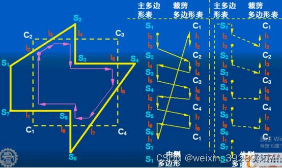
2. Weiler-Atherton polygon clipping algorithm
Main Polymorph: The polygon used to be clipped, which can be convex, concave, or with holes Clipped
Polygon: The polygon used to clip the main polygon, which can be convex, concave, or defined with
holes Direction of polygons: Clockwise direction for outer polygons, counterclockwise direction for inner polygons
Entry point: Intersection point when entering from the main polygon into the interior of the clipping polygon
Out point: Intersection point when leaving the interior of the clipping polygon
from the main polygon Start at the entry point, track along the boundary of the main polygon until you find the intersection point (out point) with the clipping polygon, turn right at the intersection point, and track along the boundary of the main polygon again; repeat the above process until you return to the algorithm
Main terminology and data structure of the Weiler-Atherton polygon clipping algorithm from the starting point of intersection (entry point)
Vertex table of the main polygon: used to define the main polygon
Vertex table of the clipped polygon: used to define the clipped polygon
Entry point table: contains The intersection point where the main polygon enters the interior of the clipping polygon.
Out point table: Contains the intersection points of the main polygon when it leaves the interior of the clip polygon
Inner table of polygons: The boundaries of the main polygon that lie inside the clip polygon and the boundaries of the clip polygons that lie inside the main polygon (which form the holes of the main polygon)
Polygons is a table of: the bounds of the main polygon outside the clipping polygon and the bounds of the clipping polygon inside the main polygon, but not including the bounds of the clipping polygon outside the main polygon
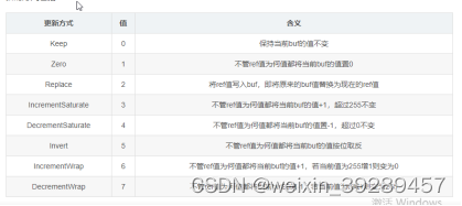
2. Template test
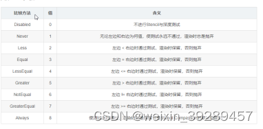
Next is template testing. This step compares the reference value provided by our app to the contents of the stencil cache, which stores a value for each pixel. If the stencil test is enabled, the GPU will first read (use the read mask) the stencil value of the fragment position in the stencil buffer, and then compare the value with the read (use the read mask) to the reference value (reference vale) for comparison, this comparison function can be specified by the developer. If the fragment fails this test, the fragment will be discarded, which is the condition for judging whether to keep it when rendering
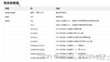
Stencil Comparison . After the Stencil Operation rendering test, regardless of whether the pixel is finally retained or discarded, the Stencil Operation will be executed to update the value in the buffer stencilBufferValue. The specific update methods include:
2. Depth test (blanking)
Since the depth information is lost by the projection transformation, it often leads to the ambiguity of the graphics. To eliminate ambiguity, lines and areas that are not actually visible must be hidden when drawing, that is, hidden. The hidden projection image is called the real image of the object.
Realization Space of Concealment Algorithm: Concealment algorithm can be implemented in object space or image space.
1.z buffer algorithm
The z-buffer algorithm is the simplest hidden surface concealment algorithm among all image space algorithms. The z-buffer algorithm is an operation that compares the z-coordinate of the fragment with the contents of the depth buffer. The depth buffer is a memory area that is part of the frame buffer just like the stencil buffer. It stores a value for each pixel, and the buffer contains the depth of each pixel. In general, the depth buffer value ranges from 0 to 1, where it represents the nearest point in the depth buffer, and 1 represents the farthest point. To determine whether a fragment is closer than other fragments already rendered at the same location, Opengl compares the z component of the fragment's window coordinates with the fragment's value already in the depth buffer. If the value is less than what is already in the cache, the fragment is visible. The meaning of this test can also change. For example, we can order Opengl to pass through fragments whose z coordinates are greater than, equal to, or not equal to the depth buffer content.
Algorithm Analysis
Simple, easy to handle hidden surfaces and display intersecting lines between surfaces. The displayed picture can be arbitrarily complex, because the size of the image space is fixed, and the calculation amount increases linearly with the complexity of the picture in the worst case, because the displayed elements can be written into the frame buffer and z buffer in any order, so Depth sorting is not required, saving sorting time
Disadvantages: A z buffer that takes up a lot of storage space is required. If the z value of the image to be displayed changes within a certain range after transformation and clipping, a fixed precision z buffer can be used. Buffer, this algorithm can produce better results after combining lighting, transparency and other related algorithms
2.Roberts algorithm
The Roberts concealment algorithm is a concealment algorithm implemented in object space. The number processing is rigorous, and the amount of calculation is very large. The Roberts algorithm requires that all displayed objects are convex, so the concave body must first be divided into a combination of many convex bodies. The specific details are more complicated, you can understand them yourself, and will not expand them in detail.
Algorithm steps
1. Consider each object independently one by one, and find out the edges and faces occluded by itself
2. Compare the edges left on each object with other objects one by one to determine whether it is completely visible It is still partially or partially occluded
3. Determine whether it is necessary to form a new display edge due to the mutual penetration between objects, etc., so that the displayed objects are closer to the display. The Roberts blanking algorithm is a blanking algorithm implemented in the image
space , the mathematical processing is rigorous, and the amount of calculation is very large. The Roberts algorithm requires that all displayed objects are convex, so the concave body must first be divided into a combination of many convex bodies.
2. Warnock algorithm
Consider a window in image space, determine whether the window is empty, or whether the pictures contained in the window are simple enough to be displayed immediately, otherwise, split the window until all contained pictures in the sub-window are sufficiently simple to be displayed immediately or the size has reached the given resolution.
Conditions for the picture to be simple enough
1. The window contains only one polygon
2. The window intersects with a polygon and there are no other polygons in the window
3. The window is surrounded by a polygon and there are no other polygons in the window
4. The window is surrounded by at least one polygon And this polygon is closest to the view point
The relationship between the polygon and the window
Warnock algorithm is divided into 5 parts
Control program: control the detection window, when the detection fails, continue to divide the window to ensure that the entire screen is detected
Detection program: check all objects All polygons, divide them into separating, enclosing, contained and intersecting polygons, and create three tables, enclosing polygons table, separating polygons table, intersecting and contained polygons table, for further processing by the analysis program Analysis program: Provided by the analysis check
program Information, analysis results, the screen is simple enough, call the computer to display, the screen is complex, declare failure, empty window, no need to process Calculation display: After
clipping, the visible part of the display window
is displayed. Display: When the window contains only one raster point, one The most critical part of the point
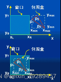
WarNock algorithm is to check the program to determine whether a polygon is separated from the window, contains, intersects or encloses. The method of judging the relationship between the polygon and the window will be introduced in detail below. Polygon separation window discrimination: For rectangular windows, bounding boxes can be
used or the maxmin test method has decided whether the polygon is separated from the window
Suppose Xl, Xr, Yr, Yl define the four sides of the window, Xmin, Ymin, Xmax, Ymax define a polygon bounding box, when the following conditions are met, the polygon is separated from the window: Xmin > Xr or Xmax < Xl or Ymin > Yl or Ymax < Yr
The discrimination of the polygon contained in the window: When the polygon bounding box is contained in the window, that is, the condition Xmin >= Xr and Xmax <= Xr and Ymin >= Yr and Ymax <= Yl The discrimination of the intersection of the polygon and the window can
be Use the straight line equation as the discriminant function to determine whether a polygon intersects with the window.
Assume that the two vertices of one side of the polygon are P1(X1, Y1) P2(X2, Y2), and the straight line equation is y = kx + b(x1 ! = x2)
then the discriminant function of the straight line is TF = y - kx - b or TF = X -X1 (X1 = X2)
among them, k = (y2 - y1)/(x2 - x1), b = y1 - kx1
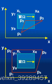
discriminant step Substituting the discriminant function for each vertex of the window as follows
, if the signs of the discriminant function values of all vertices are the same, then all points are located on the same side of the polygon edge, that is, the edge does not intersect with the window; otherwise, the line where the edge is located is the same as Window intersection is simply regarded as the intersection of a polygon and a window.
If each edge of the polygon does not intersect the window, the polygon is either separated from the window or encloses the window
The further discrimination of the separation and enclosing polygons can be carried out by using the transfer cumulative inspection method
to accumulate the angles formed by the start and end points of each side of the polygon to any point in the window in a clockwise or counterclockwise manner around the polygon, and judge according to the sum of the accumulated angles.
If the sum of the angles is equal to 0, it means that the polygon is separated from the window.
If the sum of the angles is equal to ±360*n, it means that the polygon encloses the window (n times).
Depth
calculation is required for the enclosing polygon. Compare the angles of each polygon plane in the window The depth at the point (z coordinate)
on the left shows a situation where extending the plane where the polygon is located to the window boundary may lead to a judgment error that the enclosing polygon blocks other polygons. Therefore, this situation needs to be further judged by continuing to divide the window.
The figure on the right shows another situation: extend the plane where the polygon is located to the boundary of the window, and there is no intersection with the enclosing polygon in the window, and there will be no discrimination error that the enclosing polygon blocks other polygons, so this situation belongs to the picture is simple enough, not window needs to be split
3. Table priority algorithm
The depth priority table is performed according to the distance of each element to be displayed from the viewpoint. When the algorithm is executed, starting from the element farthest from the viewpoint, each element is written into the frame buffer in turn, and finally the content in the frame buffer is always covered by elements closer to the viewpoint
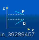
. Relationship between two polygons P and Q in sort. Polygons can be sorted by their maximum or minimum z value. Let’s assume that the maximum z value of polygons is sorted Zmax§ > Zmax(Q), that is, P is ranked before Q in the priority. As shown in the upper right figure: P and Q two planes satisfy
Zmax § > Zmax(Q), then it can be directly displayed according to the priority order of the list.
As shown in the lower right figure: Although P is ranked before Q in the priority table, if P and Q are respectively written into the frame buffer for display in this order, the Q part will cover P, and in fact It is part of P that occludes Q, so the values of P and Q must be swapped in the priority table
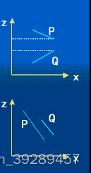
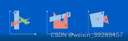
The above figure shows several other complicated situations, and it is impossible to establish a correct depth-first table. The solution is to divide these polygons circularly along the intersection line between the planes where the polygons are located, and finally determine their priority table completely (see the dotted line. )
3. mix
Fragments that pass the depth test go to the next stage - blending.
For opaque objects, develop this to turn off the blending operation. In this way, the color value calculated by the fragment shader will directly overwrite the pixel value in the color buffer. But for translucent objects, we need a blending operation to make the object look transparent. The GPU takes the source and destination colors and mixes the two colors. The source color refers to the color value obtained by the fragment shader, and the destination color is the color already existing in the color buffer. Afterwards, a blending function is used to perform the blending operation. This blending function is usually closely related to the transparent channel, such as adding, subtracting, multiplying, etc. according to the value of the transparent channel.
Common Blend Types
Blend SrcAlpha OneMinusSrcAlpha // Traditional Transparency
Blend One OneMinusSrcAlpha // Premultiplied Transparency
Blend One One // Additive
Blend OneMinusDstColor One // Soft Additive
Blend DstColor Zero // Multiplicative
Blend DstColor SrcColor // 2x Multiplicative
4. Logical operations
Fragment colors are sent to logic operations stage and finally displayed on screen
Summarize
The above is the basic content of the general graphics pipeline. In the future, I may continue to write the matrix, part of the shader data interaction.
quote
OpenGL Super Collection
bilibili Shanghai Jiaotong University Graphics