Generative Adversarial Networks
Throughout most of this book, we have talked about how to make predictions. In some form or another, we used deep neural networks learned mappings from data points to labels. This kind of learning is called discriminative learning, as in, we’d like to be able to discriminate between photos cats and photos of dogs. Classifiers and regressors are both examples of discriminative learning. And neural networks trained by backpropagation have upended everything we thought we knew about discriminative learning on large complicated datasets. Classification accuracies on high-res images has gone from useless to human-level (with some caveats) in just 5-6 years. We will spare you another spiel about all the other discriminative tasks where deep neural networks do astoundingly well.在本书的大部分内容中,我们都讨论了如何进行预测。在某种形式上,我们使用了深度神经网络学习的从数据点到标签的映射。这种学习称为判别学习,例如,我们希望能够区分照片中的猫和狗中的照片。分类器和回归器都是歧视性学习的例子。通过反向传播训练的神经网络颠覆了我们认为关于大型复杂数据集的判别式学习的所有知识。在短短5至6年间,高分辨率图像的分类精度已从无用变成了人类级别(有些警告)。我们将不为您所困扰,因为深度神经网络的所有其他判别任务都表现出色。
But there is more to machine learning than just solving discriminative tasks. For example, given a large dataset, without any labels, we might want to learn a model that concisely captures the characteristics of this data. Given such a model, we could sample synthetic data points that resemble the distribution of the training data. For example, given a large corpus of photographs of faces, we might want to be able to generate a new photorealistic image that looks like it might plausibly have come from the same dataset. This kind of learning is called generative modeling.但是,机器学习不仅仅是解决区分性任务。例如,给定一个大型数据集,而没有任何标签,我们可能想要学习一个简洁地捕获此数据特征的模型。给定这样一个模型,我们可以对类似于训练数据分布的综合数据点进行采样。例如,给定大量的面孔照片,我们可能希望能够生成新的真实感图像,看起来好像它可能来自同一数据集。这种学习称为生成建模。
Until recently, we had no method that could synthesize novel photorealistic images. But the success of deep neural networks for discriminative learning opened up new possibilities. One big trend over the last three years has been the application of discriminative deep nets to overcome challenges in problems that we do not generally think of as supervised learning problems. The recurrent neural network language models are one example of using a discriminative network (trained to predict the next character) that once trained can act as a generative model.直到最近,我们还没有能够合成新颖的逼真的图像的方法。但是,深度神经网络用于判别学习的成功开辟了新的可能性。在过去三年中,一大趋势是应用区分性深网来克服我们通常不认为是监督学习的问题中的挑战。递归神经网络语言模型是使用判别网络(经过训练可预测下一个字符)的一个示例,该网络一旦受过训练就可以充当生成模型。
In 2014, a breakthrough paper introduced Generative adversarial networks (GANs) Goodfellow.Pouget-Abadie.Mirza.ea.2014, a clever new way to leverage the power of discriminative models to get good generative models. At their heart, GANs rely on the idea that a data generator is good if we cannot tell fake data apart from real data. In statistics, this is called a two-sample test - a test to answer the question whether datasets X={x1,…,xn} and X’={x’1,…,x’n} were drawn from the same distribution. The main difference between most statistics papers and GANs is that the latter use this idea in a constructive way. In other words, rather than just training a model to say “hey, these two datasets do not look like they came from the same distribution”, they use the two-sample test to provide training signals to a generative model. This allows us to improve the data generator until it generates something that resembles the real data. At the very least, it needs to fool the classifier. Even if our classifier is a state of the art deep neural network.2014年,一篇突破性论文介绍了Generative Adversarial Network(GANs)Goodfellow.Pouget-Abadie.Mirza.ea.2014,这是一种利用判别模型的力量来获得良好的生成模型的聪明新方法。 GAN的核心思想是,如果我们不能将假数据与真实数据区分开,那么数据生成器就很好。在统计中,这称为两次抽样检验-回答数据集X = {x1,…,xn}和X ’ = {x '1, …,x 'n}来自同一分布。大多数统计文件与GAN之间的主要区别在于,后者以建设性的方式使用了这一思想。换句话说,他们不只是训练模型说“嘿,这两个数据集看起来好像不是来自相同的分布”,而是使用两个样本的检验为生成的模型提供训练信号。这使我们能够改进数据生成器,直到它生成类似于真实数据的内容为止。至少,它需要愚弄分类器。即使我们的分类器是最先进的深度神经网络。

The GAN architecture is illustrated.As you can see, there are two pieces in GAN architecture - first off, we need a device (say, a deep network but it really could be anything, such as a game rendering engine) that might potentially be able to generate data that looks just like the real thing. If we are dealing with images, this needs to generate images. If we are dealing with speech, it needs to generate audio sequences, and so on. We call this the generator network. The second component is the discriminator network. It attempts to distinguish fake and real data from each other. Both networks are in competition with each other. The generator network attempts to fool the discriminator network. At that point, the discriminator network adapts to the new fake data. This information, in turn is used to improve the generator network, and so on.可以看到GAN架构。正如您所看到的,GAN架构有两部分-首先,我们需要一个设备(例如,深层网络,但实际上可能是任何东西,例如游戏渲染引擎),这可能是能够生成看起来像真实事物的数据。如果要处理图像,则需要生成图像。如果要处理语音,则需要生成音频序列,依此类推。我们称其为生成器网络。第二部分是鉴别器网络。它试图将伪造数据与真实数据区分开。这两个网络相互竞争。生成器网络试图欺骗鉴别器网络。此时,鉴别器网络将适应新的伪造数据。该信息继而用于改善生成器网络,等等。
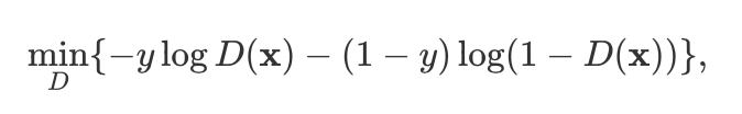
The discriminator is a binary classifier to distinguish if the input x is real (from real data) or fake (from the generator). Typically, the discriminator outputs a scalar prediction o ∈ R for input , such as using a dense layer with hidden size 1, and then applies sigmoid function to obtain the predicted probability D(x) = 1/(1+e-o). Assume the label y for the true data is 1 and 0 for the fake data. We train the discriminator to minimize the cross-entropy loss, i.e.,鉴别器是一个二进制分类器,用于区分输入x是真实的(来自真实数据)还是伪造的(来自生成器)。通常,鉴别器为输入输出标量预测o∈R,例如使用具有隐藏大小1的密集层,然后应用S型函数来获得预测概率D(x)= 1 /(1 + e ^ -o ^ )。假设真实数据的标签y为1,伪数据的标签为0。我们训练鉴别器以最小化交叉熵损失,即
For the generator, it first draws some parameter z ∈ Rd from a source of randomness, e.g., a normal distribution z ~ N(0,1). We often call z as the latent variable. It then applies a function to generate x’ = G(z). The goal of the generator is to fool the discriminator to classify x’ = G(z) as true data, i.e., we want D(G(z)) ≈ 1. In other words, for a given discriminator D, we update the parameters of the generator G to maximize the cross-entropy loss when y = 0, i.e.,对于生成器,它首先从随机性源(例如正态分布z〜N(0,1))中绘制一些参数z∈R ^ d ^。我们通常称z为潜在变量。然后,它应用一个函数来生成x ’ = G(z)。生成器的目的是欺骗鉴别器,将x ’ = G(z)分类为真实数据,即,我们希望D(G(z))≈1。换句话说,对于给定的鉴别器D,我们当y = 0时,更新发生器G的参数以最大化交叉熵损失,即
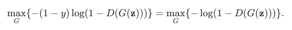
If the discriminator does a perfect job, then D(x’) ≈ 0 so the above loss near 0, which results the gradients are too small to make a good progress for the generator. So commonly we minimize the following loss:如果判别器做得很完美,则D(x ')≈0,因此上述损失接近0,这导致梯度太小而无法为发生器带来良好的进展。因此,通常我们将以下损失降到最低:
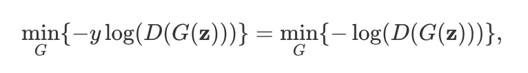
which is just feed x’ = G(z) into the discriminator but giving label y = 1.这只是将x ’ = G(z)馈入鉴别器,但给定标签y = 1。
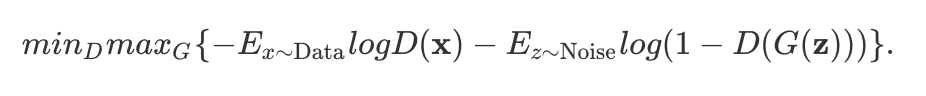
To sum up, D and G are playing a “minimax” game with the comprehensive objective function:总而言之,D和G正在玩具有综合目标功能的“极大极小”游戏:
Many of the GANs applications are in the context of images. As a demonstration purpose, we are going to content ourselves with fitting a much simpler distribution first. We will illustrate what happens if we use GANs to build the world’s most inefficient estimator of parameters for a Gaussian. Let’s get started.许多GAN应用程序都在图像环境中。作为演示目的,我们将首先满足于简化简单的发行版。我们将说明如果使用GAN为高斯建立世界上效率最低的参数估计器,将会发生什么情况。让我们开始吧。
%matplotlib inline
import matplotlib.pyplot as plt
from torch.utils.data import DataLoader
from torch import nn
import numpy as np
from torch.autograd import Variable
import torch
Generate some “real” data
Since this is going to be the world’s lamest example, we simply generate data drawn from a Gaussian.由于这将是世界上最繁琐的示例,因此我们只需要从高斯生成数据即可。
X=np.random.normal(size=(1000,2))
A=np.array([[1,2],[-0.1,0.5]])
b=np.array([1,2])
data=X.dot(A)+b
Let’s see what we got. This should be a Gaussian shifted in some rather arbitrary way with mean b and covariance matrix ATA.让我们看看我们得到了什么。这应该是以均值b和协方差矩阵ATA以某种相当随意的方式进行的高斯移位。
plt.figure(figsize=(3.5,2.5))
plt.scatter(X[:100,0],X[:100,1],color='red')
plt.show()
plt.figure(figsize=(3.5,2.5))
plt.scatter(data[:100,0],data[:100,1],color='blue')
plt.show()
print("The covariance matrix is\n%s" % np.dot(A.T, A))


The covariance matrix is
[[1.01 1.95]
[1.95 4.25]]
batch_size=8
data_iter=DataLoader(data,batch_size=batch_size)
Generator
Our generator network will be the simplest network possible - a single layer linear model. This is since we will be driving that linear network with a Gaussian data generator. Hence, it literally only needs to learn the parameters to fake things perfectly.我们的生成器网络将是最简单的网络-单层线性模型。这是因为我们将使用高斯数据生成器来驱动线性网络。因此,它实际上只需要学习参数就可以完美地伪造事物。
class net_G(nn.Module):
    def __init__(self):
        super(net_G,self).__init__()
        self.model=nn.Sequential(
            nn.Linear(2,2),
        )
        self._initialize_weights()
    def forward(self,x):
        x=self.model(x)
        return x
    def _initialize_weights(self):
        for m in self.modules():
            if isinstance(m,nn.Linear):
                m.weight.data.normal_(0,0.02)
                m.bias.data.zero_()
Discriminator
For the discriminator we will be a bit more discriminating: we will use an MLP with 3 layers to make things a bit more interesting.对于区分器,我们将更具区分性:我们将使用具有3层的MLP来使事情变得更有趣。
class net_D(nn.Module):
    def __init__(self):
        super(net_D,self).__init__()
        self.model=nn.Sequential(
            nn.Linear(2,5),
            nn.Tanh(),
            nn.Linear(5,3),
            nn.Tanh(),
            nn.Linear(3,1),
            nn.Sigmoid()
        )
        self._initialize_weights()
    def forward(self,x):
        x=self.model(x)
        return x
    def _initialize_weights(self):
        for m in self.modules():
            if isinstance(m,nn.Linear):
                m.weight.data.normal_(0,0.02)
                m.bias.data.zero_()
Training
First we define a function to update the discriminator.首先,我们定义一个函数来更新鉴别器。
# Saved in the d2l package for later use
def update_D(X,Z,net_D,net_G,loss,trainer_D):
    batch_size=X.shape[0]
    Tensor=torch.FloatTensor
    ones=Variable(Tensor(np.ones(batch_size))).view(batch_size,1)
    zeros = Variable(Tensor(np.zeros(batch_size))).view(batch_size,1)
    real_Y=net_D(X.float())
    fake_X=net_G(Z)
    fake_Y=net_D(fake_X)
    loss_D=(loss(real_Y,ones)+loss(fake_Y,zeros))/2
    loss_D.backward()
    trainer_D.step()
    return float(loss_D.sum())
The generator is updated similarly. Here we reuse the cross-entropy loss but change the label of the fake data from 0 to 1.生成器的更新类似。在这里,我们重复使用交叉熵损失,但将伪数据的标签从0更改为1。
# Saved in the d2l package for later use
def update_G(Z,net_D,net_G,loss,trainer_G):
    batch_size=Z.shape[0]
    Tensor=torch.FloatTensor
    ones=Variable(Tensor(np.ones((batch_size,)))).view(batch_size,1)
    fake_X=net_G(Z)
    fake_Y=net_D(fake_X)
    loss_G=loss(fake_Y,ones)
    loss_G.backward()
    trainer_G.step()
    return float(loss_G.sum())
Both the discriminator and the generator performs a binary logistic regression with the cross-entropy loss. We use Adam to smooth the training process. In each iteration, we first update the discriminator and then the generator. We visualize both losses and generated examples.
鉴别器和生成器都执行具有交叉熵损失的二进制逻辑回归。我们使用Adam来简化培训过程。在每次迭代中,我们首先更新鉴别器,然后更新生成器。我们将损失和生成的示例可视化。
def train(net_D,net_G,data_iter,num_epochs,lr_D,lr_G,latent_dim,data):
    loss=nn.BCELoss()
    Tensor=torch.FloatTensor
    trainer_D=torch.optim.Adam(net_D.parameters(),lr=lr_D)
    trainer_G=torch.optim.Adam(net_G.parameters(),lr=lr_G)
    plt.figure(figsize=(7,4))
    d_loss_point=[]
    g_loss_point=[]
    d_loss=0
    g_loss=0
    for epoch in range(1,num_epochs+1):
        d_loss_sum=0
        g_loss_sum=0
        batch=0
        for X in data_iter:
            batch+=1
            X=Variable(X)
            batch_size=X.shape[0]
            Z=Variable(Tensor(np.random.normal(0,1,(batch_size,latent_dim))))
            trainer_D.zero_grad()
            d_loss = update_D(X, Z, net_D, net_G, loss, trainer_D)
            d_loss_sum+=d_loss
            trainer_G.zero_grad()
            g_loss = update_G(Z, net_D, net_G, loss, trainer_G)
            g_loss_sum+=g_loss
        d_loss_point.append(d_loss_sum/batch)
        g_loss_point.append(g_loss_sum/batch)
    plt.ylabel('Loss', fontdict={'size': 14})
    plt.xlabel('epoch', fontdict={'size': 14})
    plt.xticks(range(0,num_epochs+1,3))
    plt.plot(range(1,num_epochs+1),d_loss_point,color='orange',label='discriminator')
    plt.plot(range(1,num_epochs+1),g_loss_point,color='blue',label='generator')
    plt.legend()
    plt.show()
    print(d_loss,g_loss)

    Z =Variable(Tensor( np.random.normal(0, 1, size=(100, latent_dim))))
    fake_X=net_G(Z).detach().numpy()
    plt.figure(figsize=(3.5,2.5))
    plt.scatter(data[:,0],data[:,1],color='blue',label='real')
    plt.scatter(fake_X[:,0],fake_X[:,1],color='orange',label='generated')
    plt.legend()
    plt.show()
Now we specify the hyper-parameters to fit the Gaussian distribution.
现在,我们指定超参数以适合高斯分布。
if __name__ == '__main__':
    lr_D,lr_G,latent_dim,num_epochs=0.05,0.005,2,20
    generator=net_G()
    discriminator=net_D()
    train(discriminator,generator,data_iter,num_epochs,lr_D,lr_G,latent_dim,data)

0.6932446360588074 0.6927103996276855

Summary
- Generative adversarial networks (GANs) composes of two deep networks, the generator and the discriminator.生成对抗网络(GANs)由两个深层网络组成,即生成器和鉴别器。
- The generator generates the image as much closer to the true image as possible to fool the discriminator, via maximizing the cross-entropy loss, i.e., max log(D(x’)).生成器通过最大化交叉熵损失(即max log(D(x ')))来生成尽可能接近真实图像的图像,以欺骗鉴别器。
- The discriminator tries to distinguish the generated images from the true images, via minimizing the cross-entropy loss, i.e., min - log(D(x)) - (1-y)log(1-D(x)).鉴别器试图通过最小化交叉熵损失,即min-log(D(x))-(1-y)log(1-D(x)),来将生成的图像与真实图像区分开。
