【TensorFlow】实现简单的鸢尾花分类器

代码实现及说明

# python 3.6
# TensorFlow实现简单的鸢尾花分类器
import matplotlib.pyplot as plt
import tensorflow as tf
import numpy as np
from sklearn import datasets

sess = tf.Session()

#导入数据
iris = datasets.load_iris()
# 是否是山鸢尾 0/1
binary_target = np.array([1. if x == 0 else 0. for
                            x in iris.target])
# 选择两个特征：花瓣长度和宽度
iris_2d = np.array([[x[2],x[3]] for x in iris.data])

# 声明批训练大小、占位符和变量
# tf.float32降低float字节数 可以提高算法性能
batch_size = 20
x1_data = tf.placeholder(shape=[None,1],dtype=tf.float32)
x2_data = tf.placeholder(shape=[None,1],dtype=tf.float32)
y_target = tf.placeholder(shape=[None,1],dtype=tf.float32)
# 声明变量 A 和 b (0 = x1 - A*x2 + b)
A = tf.Variable(tf.random_normal(shape=[1,1]))
b = tf.Variable(tf.random_normal(shape=[1,1]))

# 定义线性模型
# 线性模型的表达式为：x1=x2*A+b。
# 如果找到的数据点在直线以上，则将数据点代入x1-x2*A-b计算出的结果大于0；
# 同理找到的数据点在直线以下，则将数据点代入x1-x2*A-b计算出的结果小于0。
# 将公式x1-x2*A-b传入sigmoid函数，然后预测结果1或者0
# TensorFlow有内建的sigmoid损失函数，所以这里仅仅需要定义模型输出
my_mult = tf.matmul(x2_data, A)
my_add = tf.add(my_mult, b)
my_output = tf.subtract(x1_data,my_add)

# 增加分类损失函数 这里用两类交叉熵损失函数 cross entropy
xentropy = tf.nn.sigmoid_cross_entropy_with_logits(logits=my_output,labels=y_target)

# 声明优化器
my_opt = tf.train.GradientDescentOptimizer(0.05)
train_step = my_opt.minimize(xentropy)

# 初始化变量
init = tf.global_variables_initializer()
sess.run(init)

# 循环
for i in range(1000):
    rand_index = np.random.choice(len(iris_2d),size=batch_size)
    rand_x = iris_2d[rand_index]
    rand_x1 = np.array([[x[0]] for x in rand_x])
    rand_x2 = np.array([[x[1]] for x in rand_x])
    rand_y = np.array([[y] for y in binary_target[rand_index]])
    sess.run(train_step, feed_dict={x1_data:rand_x1,x2_data:rand_x2,y_target:rand_y})
    if (i+1)%200 == 0:
        print('Step #' + str(i+1) + ' A = ' + str(sess.run(A)) + ', b = ' + str(sess.run(b)))

# 结果可视化
[[slope]] = sess.run(A) # 斜率
# 因为A的shape是(1,1)所以要写成一行一列的形式
[[intercept]] = sess.run(b) # 截距

# 创建拟合线
x = np.linspace(0, 3, num=50) # 0~3 50个均匀间隔的数字
ablineValues = []
for i in x:
  ablineValues.append(slope*i+intercept)

# 绘图
setosa_x = [a[1] for i,a in enumerate(iris_2d) if binary_target[i]==1]
setosa_y = [a[0] for i,a in enumerate(iris_2d) if binary_target[i]==1]
non_setosa_x = [a[1] for i,a in enumerate(iris_2d) if binary_target[i]==0]
non_setosa_y = [a[0] for i,a in enumerate(iris_2d) if binary_target[i]==0]
plt.plot(setosa_x, setosa_y, 'rx', ms=10, mew=2, label='setosa')
plt.plot(non_setosa_x, non_setosa_y, 'ro', label='Non-setosa')
plt.plot(x, ablineValues, 'b-')
plt.xlim([0.0, 2.7])
plt.ylim([0.0, 7.1])
plt.xlabel('Petal Length')
plt.ylabel('Petal Width')
plt.legend(loc='lower right')
plt.show()

绘图结果

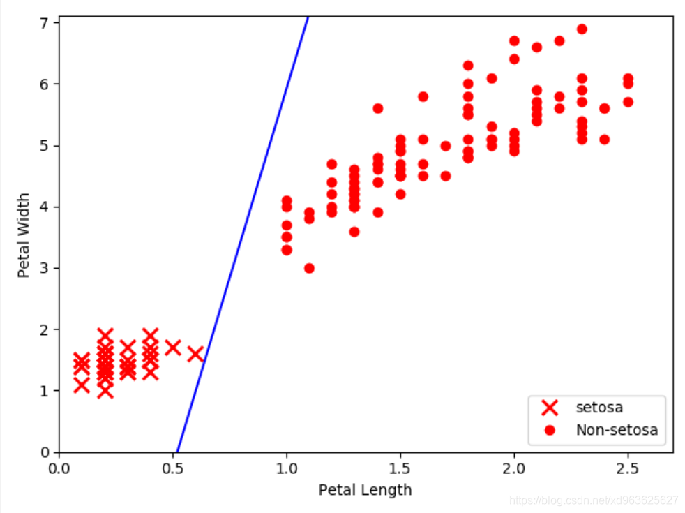
总结

这里利用花瓣长度和花瓣宽度的特征在山鸢尾与其他物种间拟合一条直线，然后通过该直线来分割两类目标（山鸢尾和非山鸢尾），直线是迭代1000次得到的线性分割，通过直线分割两个目标并不是最好的模型。