使用不同的机器学习方法进行预测
续上篇2_Linear Regression and Support Vector Regression
高斯过程回归
%matplotlib inline

import requests
from StringIO import StringIO
import numpy as np
import pandas as pd # pandas
import matplotlib.pyplot as plt # module for plotting
import datetime as dt # module for manipulating dates and times
import numpy.linalg as lin # module for performing linear algebra operations
from __future__ import division
import matplotlib

import sklearn.decomposition
import sklearn.metrics
from sklearn import gaussian_process
from sklearn import cross_validation

pd.options.display.mpl_style = 'default'
从数据预处理中读取数据
# Read in data from Preprocessing results

hourlyElectricityWithFeatures = pd.read_excel('Data/hourlyElectricityWithFeatures.xlsx')
hourlyChilledWaterWithFeatures = pd.read_excel('Data/hourlyChilledWaterWithFeatures.xlsx')
hourlySteamWithFeatures = pd.read_excel('Data/hourlySteamWithFeatures.xlsx')

dailyElectricityWithFeatures = pd.read_excel('Data/dailyElectricityWithFeatures.xlsx')
dailyChilledWaterWithFeatures = pd.read_excel('Data/dailyChilledWaterWithFeatures.xlsx')
dailySteamWithFeatures = pd.read_excel('Data/dailySteamWithFeatures.xlsx')

# An example of Dataframe
dailyChilledWaterWithFeatures.head()| chilledWater-TonDays | startDay | endDay | RH-% | T-C | Tdew-C | pressure-mbar | solarRadiation-W/m2 | windDirection | windSpeed-m/s | humidityRatio-kg/kg | coolingDegrees | heatingDegrees | dehumidification | occupancy | |
|---|---|---|---|---|---|---|---|---|---|---|---|---|---|---|---|
| 2012-01-01 | 0.961857 | 2012-01-01 | 2012-01-02 | 76.652174 | 7.173913 | 3.073913 | 1004.956522 | 95.260870 | 236.086957 | 4.118361 | 0.004796 | 0 | 7.826087 | 0 | 0.0 |
| 2012-01-02 | 0.981725 | 2012-01-02 | 2012-01-03 | 55.958333 | 5.833333 | -2.937500 | 994.625000 | 87.333333 | 253.750000 | 5.914357 | 0.003415 | 0 | 9.166667 | 0 | 0.3 |
| 2012-01-03 | 1.003672 | 2012-01-03 | 2012-01-04 | 42.500000 | -3.208333 | -12.975000 | 1002.125000 | 95.708333 | 302.916667 | 6.250005 | 0.001327 | 0 | 18.208333 | 0 | 0.3 |
| 2012-01-04 | 1.483192 | 2012-01-04 | 2012-01-05 | 41.541667 | -7.083333 | -16.958333 | 1008.250000 | 98.750000 | 286.666667 | 5.127319 | 0.000890 | 0 | 22.083333 | 0 | 0.3 |
| 2012-01-05 | 3.465091 | 2012-01-05 | 2012-01-06 | 46.916667 | -0.583333 | -9.866667 | 1002.041667 | 90.750000 | 258.333333 | 5.162041 | 0.001746 | 0 | 15.583333 | 0 | 0.3 |
以上是我们的数据样本。
每日预测:
每日用电
获取训练/验证和测试集。dataframe显示功能和目标。
def addDailyTimeFeatures(df):
    df['weekday'] = df.index.weekday
    df['day'] = df.index.dayofyear
    df['week'] = df.index.weekofyear
    return df


dailyElectricityWithFeatures = addDailyTimeFeatures(dailyElectricityWithFeatures)

df = dailyElectricityWithFeatures[['weekday', 'day', 'week',
                                   'occupancy', 'electricity-kWh']]
#df.to_excel('Data/trainSet.xlsx')
trainSet = df['2012-01':'2013-06']
testSet_dailyElectricity = df['2013-07':'2014-10']

#normalizer = np.max(trainSet)
#trainSet = trainSet / normalizer
#testSet = testSet / normalizer
trainX_dailyElectricity = trainSet.values[:,0:-1]
trainY_dailyElectricity = trainSet.values[:,4]

testX_dailyElectricity = testSet_dailyElectricity.values[:,0:-1]
testY_dailyElectricity = testSet_dailyElectricity.values[:,4]

trainSet.head()| weekday | day | week | occupancy | electricity-kWh | |
|---|---|---|---|---|---|
| 2012-01-01 | 6 | 1 | 52 | 0.0 | 2800.244977 |
| 2012-01-02 | 0 | 2 | 1 | 0.3 | 3168.974047 |
| 2012-01-03 | 1 | 3 | 1 | 0.3 | 5194.533376 |
| 2012-01-04 | 2 | 4 | 1 | 0.3 | 5354.861935 |
| 2012-01-05 | 3 | 5 | 1 | 0.3 | 5496.223993 |
以上是在预测每日用电时使用的特性。
交叉验证以获得输入参数 theta , nuggest
实际上有一些后台测试。首先做一个粗糙的网格serach参数,这里没有显示。之后,就可以得到精细网格搜索的参数范围,如下图所示。
def crossValidation_all(theta, nugget, nfold, trainX, trainY):

    thetaU = theta * 2
    thetaL = theta/2

    scores = np.zeros((len(nugget) * len(theta), nfold))
    labels = ["" for x in range(len(nugget) * len(theta))]

    k = 0
    for j in range(len(theta)):
        for i in range(len(nugget)):
            gp = gaussian_process.GaussianProcess(theta0 = theta[j], nugget = nugget[i])
            scores[k, :] = cross_validation.cross_val_score(gp,
                                                            trainX, trainY,
                                                            scoring='r2', cv = nfold)
            labels[k] = str(theta[j]) + '|' + str(nugget[i])
            k = k + 1

    plt.figure(figsize=(20,8))
    plt.boxplot(scores.T, sym='b+', labels = labels, whis = 0.5)
    plt.ylim([0,1])
    plt.title('R2 score as a function of nugget')
    plt.ylabel('R2 Score')
    plt.xlabel('Choice of theta | nugget')
    plt.show()

theta = np.arange(1, 8, 2)
nfold = 10
nugget = np.arange(0.01, 0.2, 0.03)

crossValidation_all(theta, nugget, nfold, trainX_dailyElectricity, trainY_dailyElectricity)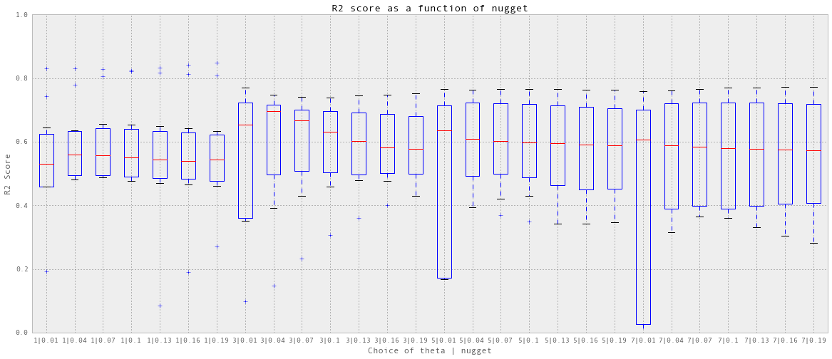
我选择theta = 3, nuggest = 0.04,这是最好的中位数预测精度。
预测,计算精度和可视化
def predictAll(theta, nugget, trainX, trainY, testX, testY, testSet, title):

    gp = gaussian_process.GaussianProcess(theta0=theta, nugget =nugget)
    gp.fit(trainX, trainY)

    predictedY, MSE = gp.predict(testX, eval_MSE = True)
    sigma = np.sqrt(MSE)

    results = testSet.copy()
    results['predictedY'] = predictedY
    results['sigma'] = sigma

    print "Train score R2:", gp.score(trainX, trainY)
    print "Test score R2:", sklearn.metrics.r2_score(testY, predictedY)

    plt.figure(figsize = (9,8))
    plt.scatter(testY, predictedY)
    plt.plot([min(testY), max(testY)], [min(testY), max(testY)], 'r')
    plt.xlim([min(testY), max(testY)])
    plt.ylim([min(testY), max(testY)])
    plt.title('Predicted vs. observed: ' + title)
    plt.xlabel('Observed')
    plt.ylabel('Predicted')
    plt.show()

    return gp, results

gp_dailyElectricity, results_dailyElectricity = predictAll(3, 0.04,
                                                           trainX_dailyElectricity,
                                                           trainY_dailyElectricity,
                                                           testX_dailyElectricity,
                                                           testY_dailyElectricity,
                                                           testSet_dailyElectricity,
                                                           'Daily Electricity')
Train score R2: 0.922109831389
Test score R2: 0.822408541698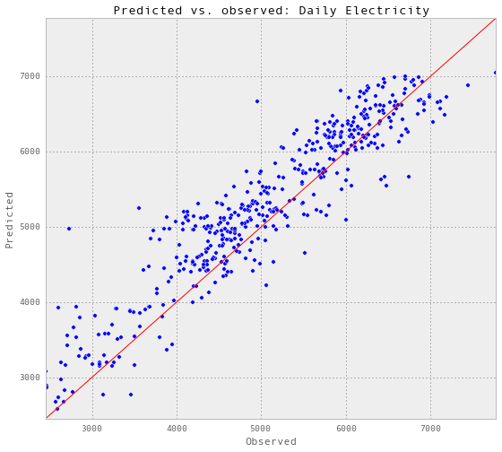

def plotGP(testY, predictedY, sigma):
    fig = plt.figure(figsize = (20,6))
    plt.plot(testY, 'r.', markersize=10, label=u'Observations')
    plt.plot(predictedY, 'b-', label=u'Prediction')
    x = range(len(testY))
    plt.fill(np.concatenate([x, x[::-1]]),
             np.concatenate([predictedY - 1.9600 * sigma,
                             (predictedY + 1.9600 * sigma)[::-1]]),
             alpha=.5, fc='b', ec='None', label='95% confidence interval')

subset = results_dailyElectricity['2013-12':'2014-06']
testY = subset['electricity-kWh']
predictedY = subset['predictedY']
sigma = subset['sigma']

plotGP(testY, predictedY, sigma)

plt.ylabel('Electricity (kWh)', fontsize = 13)
plt.title('Gaussian Process Regression: Daily Electricity Prediction', fontsize = 17)
plt.legend(loc='upper right')
plt.xlim([0, len(testY)])
plt.ylim([1000,8000])

xTickLabels = pd.DataFrame(data = subset.index[np.arange(0,len(subset.index),10)], columns=['datetime'])
xTickLabels['date'] = xTickLabels['datetime'].apply(lambda x: x.strftime('%Y-%m-%d'))
ax = plt.gca()
ax.set_xticks(np.arange(0, len(subset), 10))
ax.set_xticklabels(labels = xTickLabels['date'], fontsize = 13, rotation = 90)
plt.show()
以上是部分预测的可视化。
每日用电预测相当成功。
每日冷水
获取训练/验证和测试集。dataframe显示功能和目标。
dailyChilledWaterWithFeatures = addDailyTimeFeatures(dailyChilledWaterWithFeatures)

df = dailyChilledWaterWithFeatures[['weekday', 'day', 'week', 'occupancy',
                                    'coolingDegrees', 'T-C', 'humidityRatio-kg/kg',
                                    'dehumidification', 'chilledWater-TonDays']]
#df.to_excel('Data/trainSet.xlsx')
trainSet = df['2012-01':'2013-06']
testSet_dailyChilledWater = df['2013-07':'2014-10']

trainX_dailyChilledWater = trainSet.values[:,0:-1]
trainY_dailyChilledWater = trainSet.values[:,8]

testX_dailyChilledWater = testSet_dailyChilledWater.values[:,0:-1]
testY_dailyChilledWater = testSet_dailyChilledWater.values[:,8]

trainSet.head()| weekday | day | week | occupancy | coolingDegrees | T-C | humidityRatio-kg/kg | dehumidification | chilledWater-TonDays | |
|---|---|---|---|---|---|---|---|---|---|
| 2012-01-01 | 6 | 1 | 52 | 0.0 | 0 | 7.173913 | 0.004796 | 0 | 0.961857 |
| 2012-01-02 | 0 | 2 | 1 | 0.3 | 0 | 5.833333 | 0.003415 | 0 | 0.981725 |
| 2012-01-03 | 1 | 3 | 1 | 0.3 | 0 | -3.208333 | 0.001327 | 0 | 1.003672 |
| 2012-01-04 | 2 | 4 | 1 | 0.3 | 0 | -7.083333 | 0.000890 | 0 | 1.483192 |
| 2012-01-05 | 3 | 5 | 1 | 0.3 | 0 | -0.583333 | 0.001746 | 0 | 3.465091 |
以上是用于日常冷水预测的特征。
同样,需要对冷水进行交叉验证。
交叉验证以获得输入参数
def crossValidation(theta, nugget, nfold, trainX, trainY):

    scores = np.zeros((len(theta), nfold))

    for i in range(len(theta)):
        gp = gaussian_process.GaussianProcess(theta0 = theta[i], nugget = nugget)
        scores[i, :] = cross_validation.cross_val_score(gp, trainX, trainY, scoring='r2', cv = nfold)

    plt.boxplot(scores.T, sym='b+', labels = theta, whis = 0.5)
    #plt.ylim(ylim)
    plt.title('R2 score as a function of theta0')
    plt.ylabel('R2 Score')
    plt.xlabel('Choice of theta0')
    plt.show()
theta = np.arange(0.001, 0.1, 0.02)
nugget = 0.05
crossValidation(theta, nugget, 3, trainX_dailyChilledWater, trainY_dailyChilledWater)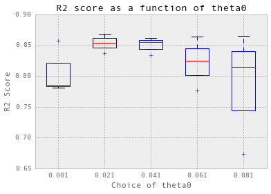
选择 theta = 0.021.
交叉验证实际上并不适用于冷冻水。首先,我必须使用三倍交叉验证,而不是十倍。此外,为了简化过程,从现在开始,我只显示针对theta的初始值的交叉验证结果:theta0。 我在后台搜索了nugget。
预测,计算精度和可视化
theta = 0.021
nugget =0.05
# Predict
gp, results_dailyChilledWater = predictAll(theta, nugget,
trainX_dailyChilledWater,
trainY_dailyChilledWater,
testX_dailyChilledWater,
testY_dailyChilledWater,
testSet_dailyChilledWater,
'Daily Chilled Water')
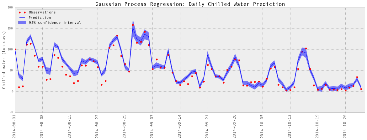
# Visualize
subset = results_dailyChilledWater['2014-08':'2014-10']
testY = subset['chilledWater-TonDays']
predictedY = subset['predictedY']
sigma = subset['sigma']
plotGP(testY, predictedY, sigma)
plt.ylabel('Chilled water (ton-days)', fontsize = 13)
plt.title('Gaussian Process Regression: Daily Chilled Water Prediction', fontsize = 17)
plt.legend(loc='upper left')
plt.xlim([0, len(testY)])
#plt.ylim([1000,8000])
xTickLabels = pd.DataFrame(data = subset.index[np.arange(0,len(subset.index),7)],
columns=['datetime'])
xTickLabels['date'] = xTickLabels['datetime'].apply(lambda x: x.strftime('%Y-%m-%d'))
ax = plt.gca()
ax.set_xticks(np.arange(0, len(subset), 7))
ax.set_xticklabels(labels = xTickLabels['date'], fontsize = 13, rotation = 90)
plt.show()Train score R2: 0.91483040513
Test score R2: 0.901408621289
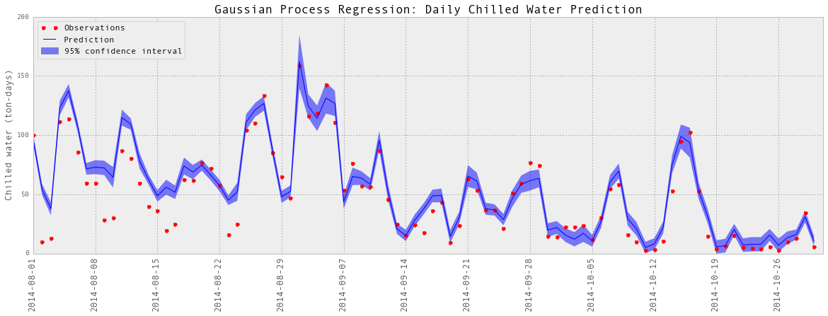
以上是部分预测的可视化。
预测又相当成功。
再增加一个特性:电量预测
为了提高预测精度,又增加了一个特性,即耗电量预测。预测的电量是根据前面电力部分中描述的时间特性产生的。这描述了入住计划。需要训练数据集中的实际用电量进行训练,然后将用电量作为测试数据集的特征进行预测。因此,这种预测方法仍然只需要时间和天气信息以及历史用电量来预测未来的用电量
dailyChilledWaterWithFeatures['predictedElectricity'] = gp_dailyElectricity.predict(
                                                            dailyChilledWaterWithFeatures[['weekday', 'day', 'week', 'occupancy']].values)

df = dailyChilledWaterWithFeatures[['weekday', 'day', 'week',
                                    'occupancy',
                                    'coolingDegrees', 'T-C',
                                    'humidityRatio-kg/kg',
                                    'dehumidification',
                                    'predictedElectricity',
                                    'chilledWater-TonDays']]
#df.to_excel('Data/trainSet.xlsx')
trainSet = df['2012-01':'2013-06']
testSet_dailyChilledWaterMoreFeatures = df['2013-07':'2014-10']

trainX_dailyChilledWaterMoreFeatures = trainSet.values[:,0:-1]
trainY_dailyChilledWaterMoreFeatures = trainSet.values[:,9]

testX_dailyChilledWaterMoreFeatures = testSet_dailyChilledWaterMoreFeatures.values[:,0:-1]
testY_dailyChilledWaterMoreFeatures = testSet_dailyChilledWaterMoreFeatures.values[:,9]

trainSet.head()| weekday | day | week | occupancy | coolingDegrees | T-C | humidityRatio-kg/kg | dehumidification | predictedElectricity | chilledWater-TonDays | |
|---|---|---|---|---|---|---|---|---|---|---|
| 2012-01-01 | 6 | 1 | 52 | 0.0 | 0 | 7.173913 | 0.004796 | 0 | 2883.784617 | 0.961857 |
| 2012-01-02 | 0 | 2 | 1 | 0.3 | 0 | 5.833333 | 0.003415 | 0 | 4231.128909 | 0.981725 |
| 2012-01-03 | 1 | 3 | 1 | 0.3 | 0 | -3.208333 | 0.001327 | 0 | 5013.703046 | 1.003672 |
| 2012-01-04 | 2 | 4 | 1 | 0.3 | 0 | -7.083333 | 0.000890 | 0 | 4985.929899 | 1.483192 |
| 2012-01-05 | 3 | 5 | 1 | 0.3 | 0 | -0.583333 | 0.001746 | 0 | 5106.976841 | 3.465091 |
交叉验证
theta = np.arange(0.001, 0.15, 0.02)
nugget = 0.05
crossValidation(theta, nugget, 3, trainX_dailyChilledWaterMoreFeatures, trainY_dailyChilledWaterMoreFeatures)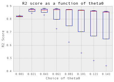
选择 theta =0.021.
预测,计算精度和可视化
# Predict
gp, results_dailyChilledWaterMoreFeatures = predictAll(
    0.021, 0.05,
    trainX_dailyChilledWaterMoreFeatures,
    trainY_dailyChilledWaterMoreFeatures,
    testX_dailyChilledWaterMoreFeatures,
    testY_dailyChilledWaterMoreFeatures,
    testSet_dailyChilledWaterMoreFeatures,
    'Daily Chilled Water')

# Visualize
subset = results_dailyChilledWaterMoreFeatures['2014-08':'2014-10']
testY = subset['chilledWater-TonDays']
predictedY = subset['predictedY']
sigma = subset['sigma']

plotGP(testY, predictedY, sigma)

plt.ylabel('Chilled water (ton-days)', fontsize = 13)
plt.title('Gaussian Process Regression: Daily Chilled Water Prediction', fontsize = 17)
plt.legend(loc='upper left')
plt.xlim([0, len(testY)])
#plt.ylim([1000,8000])

xTickLabels = pd.DataFrame(data = subset.index[np.arange(0,len(subset.index),7)],
                           columns=['datetime'])
xTickLabels['date'] = xTickLabels['datetime'].apply(lambda x: x.strftime('%Y-%m-%d'))
ax = plt.gca()
ax.set_xticks(np.arange(0, len(subset), 7))
ax.set_xticklabels(labels = xTickLabels['date'], fontsize = 13, rotation = 90)
plt.show()
Train score R2: 0.937952834542
Test score R2: 0.926978705167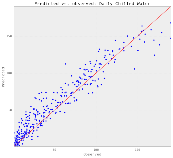
以上是部分预测的可视化。
根据R2的得分,准确性确实提高了一点。因此,我将把预测的电量包括在预测中。
热水
获取训练/验证和测试集。dataframe显示功能和目标。
dailySteamWithFeatures = addDailyTimeFeatures(dailySteamWithFeatures)

dailySteamWithFeatures['predictedElectricity'] = gp_dailyElectricity.predict(
                  dailySteamWithFeatures[['weekday', 'day', 'week', 'occupancy']].values)

df = dailySteamWithFeatures[['weekday', 'day', 'week', 'occupancy',
                             'heatingDegrees', 'T-C',
                             'humidityRatio-kg/kg', 'predictedElectricity', 'steam-LBS']]
#df.to_excel('Data/trainSet.xlsx')
trainSet = df['2012-01':'2013-06']
testSet_dailySteam = df['2013-07':'2014-10']

trainX_dailySteam = trainSet.values[:,0:-1]
trainY_dailySteam = trainSet.values[:,8]

testX_dailySteam = testSet_dailySteam.values[:,0:-1]
testY_dailySteam = testSet_dailySteam.values[:,8]

trainSet.head()| weekday | day | week | occupancy | heatingDegrees | T-C | humidityRatio-kg/kg | predictedElectricity | steam-LBS | |
|---|---|---|---|---|---|---|---|---|---|
| 2012-01-01 | 6 | 1 | 52 | 0.0 | 7.826087 | 7.173913 | 0.004796 | 2883.784617 | 17256.468099 |
| 2012-01-02 | 0 | 2 | 1 | 0.3 | 9.166667 | 5.833333 | 0.003415 | 4231.128909 | 17078.440755 |
| 2012-01-03 | 1 | 3 | 1 | 0.3 | 18.208333 | -3.208333 | 0.001327 | 5013.703046 | 59997.969401 |
| 2012-01-04 | 2 | 4 | 1 | 0.3 | 22.083333 | -7.083333 | 0.000890 | 4985.929899 | 56104.878906 |
| 2012-01-05 | 3 | 5 | 1 | 0.3 | 15.583333 | -0.583333 | 0.001746 | 5106.976841 | 45231.708984 |
交叉验证以获得输入参数
theta = np.arange(0.06, 0.15, 0.01)
nugget = 0.05
crossValidation(theta, nugget, 3, trainX_dailySteam, trainY_dailySteam)
选择theta = 0.1.
预测,计算精度和可视化
# Predict
gp, results_dailySteam = predictAll(0.1, 0.05, trainX_dailySteam, trainY_dailySteam,
                                    testX_dailySteam, testY_dailySteam, testSet_dailySteam, 'Daily Steam')

# Visualize
subset = results_dailySteam['2013-10':'2014-02']
testY = subset['steam-LBS']
predictedY = subset['predictedY']
sigma = subset['sigma']

plotGP(testY, predictedY, sigma)

plt.ylabel('Steam (LBS)', fontsize = 13)
plt.title('Gaussian Process Regression: Daily Steam Prediction', fontsize = 17)
plt.legend(loc='upper left')
plt.xlim([0, len(testY)])
#plt.ylim([1000,8000])

xTickLabels = pd.DataFrame(data = subset.index[np.arange(0,len(subset.index),10)],
                           columns=['datetime'])
xTickLabels['date'] = xTickLabels['datetime'].apply(lambda x: x.strftime('%Y-%m-%d'))
ax = plt.gca()
ax.set_xticks(np.arange(0, len(subset), 10))
ax.set_xticklabels(labels = xTickLabels['date'], fontsize = 13, rotation = 90)
plt.show()
Train score R2: 0.96729657748
Test score R2: 0.933120481633

以上是部分预测的可视化。
每小时的预测
我用同样的方法来训练和测试每小时的模型。因为随着数据点数量的增加,计算成本显著增加。在大型数据集上进行交叉验证是不可能的,因为我们没有太多的时间进行项目。因此,我只使用一小组训练/验证数据来获取参数,然后使用完整的数据集进行训练和测试,并让我的计算机连夜运行。
每小时用电量
获取训练/验证和测试集。先尝试小样本。dataframe显示特性和目标。
def addHourlyTimeFeatures(df):
    df['hour'] = df.index.hour
    df['weekday'] = df.index.weekday
    df['day'] = df.index.dayofyear
    df['week'] = df.index.weekofyear

    return df

hourlyElectricityWithFeatures = addHourlyTimeFeatures(hourlyElectricityWithFeatures)

df_hourlyElectricity = hourlyElectricityWithFeatures[['hour', 'weekday', 'day',
                                                      'week', 'cosHour',
                                                      'occupancy', 'electricity-kWh']]
#df_hourlyElectricity.to_excel('Data/trainSet_hourlyElectricity.xlsx')

def setTrainTestSets(df, trainStart, trainEnd, testStart, testEnd, indY):

    trainSet = df[trainStart : trainEnd]
    testSet = df[testStart : testEnd]

    trainX = trainSet.values[:,0:-1]
    trainY = trainSet.values[:,indY]

    testX = testSet.values[:,0:-1]
    testY = testSet.values[:,indY]

    return trainX, trainY, testX, testY, testSet

trainStart = '2013-02'
trainEnd = '2013-05'
testStart = '2014-03'
testEnd = '2014-04'

df = df_hourlyElectricity;
trainX_hourlyElectricity, trainY_hourlyElectricity, \
testX_hourlyElectricity, testY_hourlyElectricity, \
    testSet_hourlyElectricity = setTrainTestSets(df, trainStart,
                                                 trainEnd, testStart, testEnd, 6)

df_hourlyElectricity.head()| hour | weekday | day | week | cosHour | occupancy | electricity-kWh | |
|---|---|---|---|---|---|---|---|
| 2012-01-01 01:00:00 | 1 | 6 | 1 | 52 | 0.866025 | 0 | 111.479277 |
| 2012-01-01 02:00:00 | 2 | 6 | 1 | 52 | 0.965926 | 0 | 117.989395 |
| 2012-01-01 03:00:00 | 3 | 6 | 1 | 52 | 1.000000 | 0 | 119.010131 |
| 2012-01-01 04:00:00 | 4 | 6 | 1 | 52 | 0.965926 | 0 | 116.005587 |
| 2012-01-01 05:00:00 | 5 | 6 | 1 | 52 | 0.866025 | 0 | 111.132977 |
交叉验证以获得输入参数
nugget = 0.008
theta = np.arange(0.05, 0.5, 0.05)
crossValidation(theta, nugget, 10, trainX_hourlyElectricity, trainY_hourlyElectricity)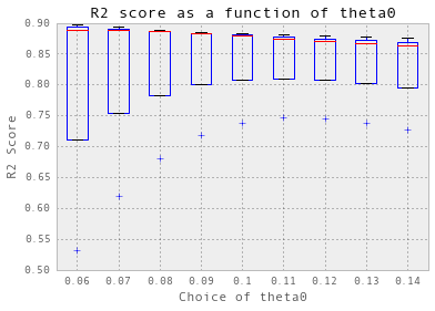
预测,计算精度和可视化
gp_hourlyElectricity, results_hourlyElectricity = predictAll(0.1, 0.008,
                                                             trainX_hourlyElectricity,
                                                             trainY_hourlyElectricity,
                                                             testX_hourlyElectricity,
                                                             testY_hourlyElectricity,
                                                             testSet_hourlyElectricity,
                                                          'Hourly Electricity (Partial)')
Train score R2: 0.957912601164
Test score R2: 0.893873175566
subset = results_hourlyElectricity['2014-03-08 23:00:00':'2014-03-15']
testY = subset['electricity-kWh']
predictedY = subset['predictedY']
sigma = subset['sigma']

plotGP(testY, predictedY, sigma)

plt.ylabel('Electricity (kWh)', fontsize = 13)
plt.title('Gaussian Process Regression: Hourly Electricity Prediction', fontsize = 17)
plt.legend(loc='upper right')
plt.xlim([0, len(testY)])
#plt.ylim([1000,8000])

xTickLabels = subset.index[np.arange(0,len(subset.index),6)]
ax = plt.gca()
ax.set_xticks(np.arange(0, len(subset), 6))
ax.set_xticklabels(labels = xTickLabels, fontsize = 13, rotation = 90)
plt.show()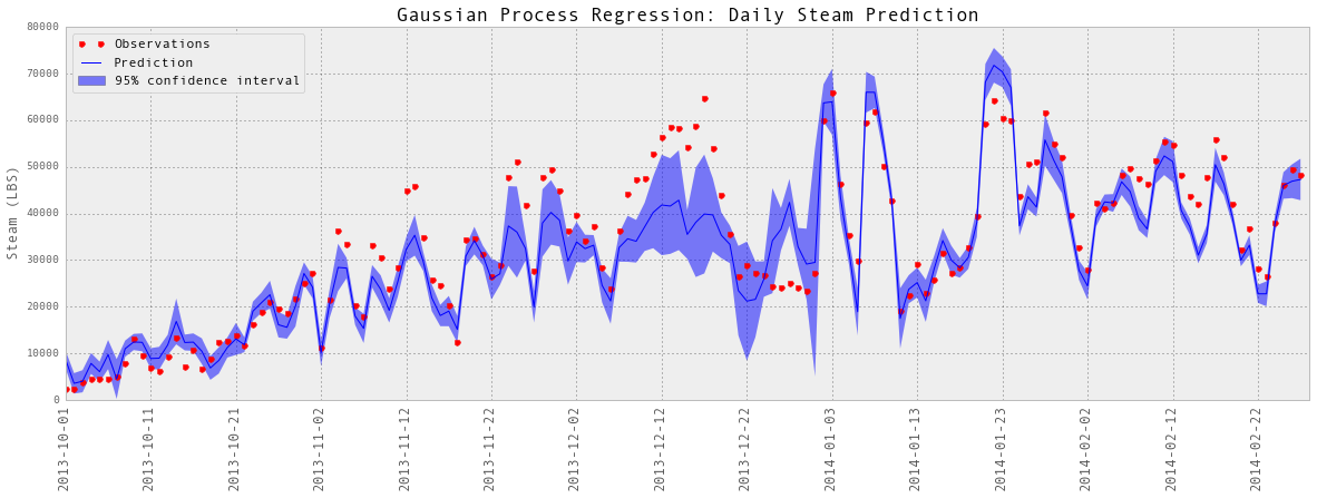
以上是部分预测的可视化。
训练和测试每小时的数据
每小时电量的最终预测精度。
trainStart = '2012-01'
trainEnd = '2013-06'
testStart = '2013-07'
testEnd = '2014-10'

results_allHourlyElectricity = pd.read_excel('Data/results_allHourlyElectricity.xlsx')

def plotR2(df, energyType, title):
    testY = df[energyType]
    predictedY = df['predictedY']

    print "Test score R2:", sklearn.metrics.r2_score(testY, predictedY)

    plt.figure(figsize = (9,8))
    plt.scatter(testY, predictedY)
    plt.plot([min(testY), max(testY)], [min(testY), max(testY)], 'r')
    plt.xlim([min(testY), max(testY)])
    plt.ylim([min(testY), max(testY)])
    plt.title('Predicted vs. observed: ' + title)
    plt.xlabel('Observed')
    plt.ylabel('Predicted')
    plt.show()

plotR2(results_allHourlyElectricity, 'electricity-kWh', 'All Hourly Electricity')
Test score R2: 0.882986662109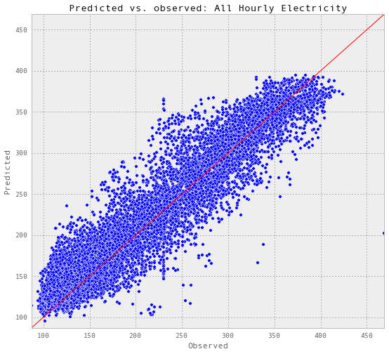
每小时用冷水
获取训练/验证和测试集。先尝试小样本。dataframe显示特性和目标。
trainStart = '2013-08'
trainEnd = '2013-10'
testStart = '2014-08'
testEnd = '2014-10'

def getPredictedElectricity(trainStart, trainEnd, testStart, testEnd):
    trainX, trainY, testX, testY, testSet = setTrainTestSets(df_hourlyElectricity,
                                                             trainStart, trainEnd,
                                                             testStart, testEnd, 6)

    gp = gaussian_process.GaussianProcess(theta0 = 0.15, nugget = 0.008)
    gp.fit(trainX, trainY)

    trainSet = df_hourlyElectricity[trainStart : trainEnd]
    predictedElectricity = pd.DataFrame(data = np.zeros(len(trainSet)),
                                        index = trainSet.index,
                                        columns = ['predictedElectricity'])
    predictedElectricity = \
    predictedElectricity.append(pd.DataFrame(data = np.zeros(len(testSet)),
                                             index = testSet.index,
                                             columns = ['predictedElectricity']))

    predictedElectricity.loc[trainStart:trainEnd,
                             'predictedElectricity'] = gp.predict(trainX)
    predictedElectricity.loc[testStart:testEnd,
                             'predictedElectricity'] = gp.predict(testX)

    return predictedElectricity

predictedElectricity = getPredictedElectricity(trainStart, trainEnd, testStart, testEnd)
hourlyChilledWaterWithMoreFeatures = \ hourlyChilledWaterWithFeatures.join(predictedElectricity, how = 'inner')

hourlyChilledWaterWithMoreFeatures = addHourlyTimeFeatures(hourlyChilledWaterWithMoreFeatures)

df_hourlyChilledWater = hourlyChilledWaterWithMoreFeatures[['hour', 'cosHour',
                                                            'weekday', 'day', 'week',
                                                            'occupancy', 'T-C',
                                                            'humidityRatio-kg/kg',
                                                            'predictedElectricity',
                                                            'chilledWater-TonDays']]

df = df_hourlyChilledWater;

trainX_hourlyChilledWater, \
trainY_hourlyChilledWater, \
testX_hourlyChilledWater,  \
testY_hourlyChilledWater, \
testSet_hourlyChilledWater = setTrainTestSets(df, trainStart, trainEnd,
                                              testStart, testEnd, 9)

df_hourlyChilledWater.head()| hour | cosHour | weekday | day | week | occupancy | T-C | humidityRatio-kg/kg | predictedElectricity | chilledWater-TonDays | |
|---|---|---|---|---|---|---|---|---|---|---|
| 2013-08-01 00:00:00 | 0 | 0.707107 | 3 | 213 | 31 | 0.5 | 17.7 | 0.010765 | 123.431454 | 0.200647 |
| 2013-08-01 01:00:00 | 1 | 0.866025 | 3 | 213 | 31 | 0.5 | 17.8 | 0.012102 | 119.266616 | 0.183318 |
| 2013-08-01 02:00:00 | 2 | 0.965926 | 3 | 213 | 31 | 0.5 | 17.7 | 0.012026 | 121.821887 | 0.183318 |
| 2013-08-01 03:00:00 | 3 | 1.000000 | 3 | 213 | 31 | 0.5 | 17.6 | 0.011962 | 124.888675 | 0.183318 |
| 2013-08-01 04:00:00 | 4 | 0.965926 | 3 | 213 | 31 | 0.5 | 17.7 | 0.011912 | 124.824413 | 0.183318 |
交叉验证以获得输入参数
nugget = 0.01
theta = np.arange(0.001, 0.05, 0.01)
crossValidation(theta, nugget, 5, trainX_hourlyChilledWater, trainY_hourlyChilledWater)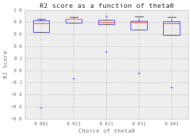
预测,计算精度和可视化
gp_hourlyChilledWater, results_hourlyChilledWater = predictAll(0.011, 0.01,
                                                               trainX_hourlyChilledWater,
                                                               trainY_hourlyChilledWater,
                                                               testX_hourlyChilledWater,
                                                               testY_hourlyChilledWater,
                                                              testSet_hourlyChilledWater,
                                                      'Hourly Chilled Water (Particial)')
Train score R2: 0.914352370778
Test score R2: 0.865202975683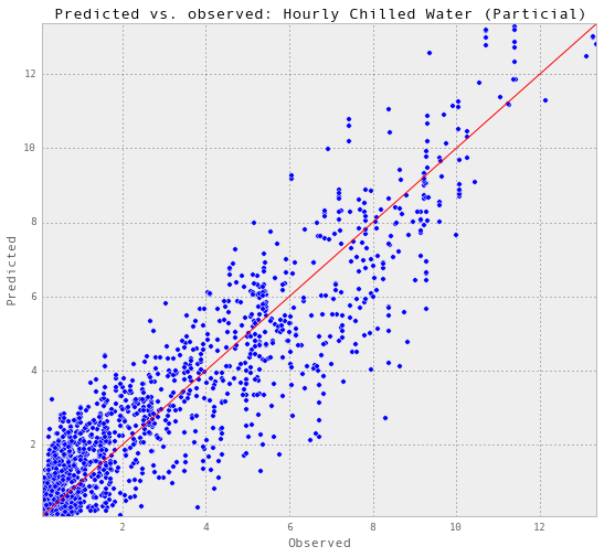
subset = results_hourlyChilledWater['2014-08-24':'2014-08-30']
testY = subset['chilledWater-TonDays']
predictedY = subset['predictedY']
sigma = subset['sigma']

plotGP(testY, predictedY, sigma)

plt.ylabel('Chilled water (ton-days)', fontsize = 13)
plt.title('Gaussian Process Regression: Hourly Chilled Water Prediction', fontsize = 17)
plt.legend(loc='upper right')
plt.xlim([0, len(testY)])
#plt.ylim([1000,8000])

xTickLabels = subset.index[np.arange(0,len(subset.index),6)]
ax = plt.gca()
ax.set_xticks(np.arange(0, len(subset), 6))
ax.set_xticklabels(labels = xTickLabels, fontsize = 13, rotation = 90)
plt.show()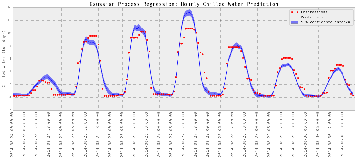
以上是部分预测的可视化。
训练和测试每小时的数据
警告:这可能需要很长时间才能执行代码。
# This could take forever.

trainStart = '2012-01'
trainEnd = '2013-06'
testStart = '2013-07'
testEnd = '2014-10'


predictedElectricity = getPredictedElectricity(trainStart, trainEnd, testStart, testEnd)
# Chilled water
hourlyChilledWaterWithMoreFeatures = hourlyChilledWaterWithFeatures.join(predictedElectricity, how = 'inner')
hourlyChilledWaterWithMoreFeatures = addHourlyTimeFeatures(hourlyChilledWaterWithMoreFeatures)

df_hourlyChilledWater = hourlyChilledWaterWithMoreFeatures[['hour', 'cosHour',
                                                            'weekday', 'day',
                                                            'week', 'occupancy', 'T-C',
                                                            'humidityRatio-kg/kg',
                                                            'predictedElectricity',
                                                            'chilledWater-TonDays']]

df = df_hourlyChilledWater;

trainX_hourlyChilledWater, \
trainY_hourlyChilledWater, \
testX_hourlyChilledWater, \
testY_hourlyChilledWater, \
testSet_hourlyChilledWater = setTrainTestSets(df, trainStart, trainEnd,
                                              testStart, testEnd, 9)

gp_hourlyChilledWater, results_hourlyChilledWater = predictAll(0.011, 0.01,
                                                               trainX_hourlyChilledWater,
                                                               trainY_hourlyChilledWater,
                                                               testX_hourlyChilledWater,
                                                               testY_hourlyChilledWater,
                                                              testSet_hourlyChilledWater)

results_hourlyChilledWater.to_excel('Data/results_allHourlyChilledWater.xlsx')
每小时冷水预报的最终精度。
results_allHourlyChilledWater = pd.read_excel('Data/results_allHourlyChilledWater.xlsx')

plotR2(results_allHourlyChilledWater, 'chilledWater-TonDays', 'All Hourly Chilled Water')
Test score R2: 0.887195665411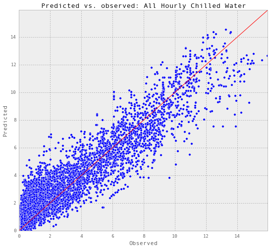
每小时用热水
获取训练/验证和测试集。先尝试小样本。dataframe显示特性和目标。
trainStart = '2012-01'
trainEnd = '2012-03'
testStart = '2014-01'
testEnd = '2014-03'

predictedElectricity = getPredictedElectricity(trainStart, trainEnd, testStart, testEnd)
hourlySteamWithMoreFeatures = hourlySteamWithFeatures.join(predictedElectricity,
                                                           how = 'inner')

hourlySteamWithMoreFeatures = addHourlyTimeFeatures(hourlySteamWithMoreFeatures)

df_hourlySteam = hourlySteamWithMoreFeatures[['hour', 'cosHour', 'weekday',
                                              'day', 'week', 'occupancy', 'T-C',
                                              'humidityRatio-kg/kg',
                                              'predictedElectricity', 'steam-LBS']]

df = df_hourlySteam;

trainX_hourlySteam,
trainY_hourlySteam,
testX_hourlySteam,
testY_hourlySteam, \
testSet_hourlySteam = setTrainTestSets(df, trainStart, trainEnd, testStart, testEnd, 9)

df_hourlySteam.head()| hour | cosHour | weekday | day | week | occupancy | T-C | humidityRatio-kg/kg | predictedElectricity | steam-LBS | |
|---|---|---|---|---|---|---|---|---|---|---|
| 2012-01-01 01:00:00 | 1 | 0.866025 | 6 | 1 | 52 | 0 | 4 | 0.004396 | 117.502720 | 513.102214 |
| 2012-01-01 02:00:00 | 2 | 0.965926 | 6 | 1 | 52 | 0 | 4 | 0.004391 | 114.720226 | 1353.371311 |
| 2012-01-01 03:00:00 | 3 | 1.000000 | 6 | 1 | 52 | 0 | 5 | 0.004380 | 113.079503 | 1494.904514 |
| 2012-01-01 04:00:00 | 4 | 0.965926 | 6 | 1 | 52 | 0 | 6 | 0.004401 | 112.428146 | 490.090061 |
| 2012-01-01 05:00:00 | 5 | 0.866025 | 6 | 1 | 52 | 0 | 4 | 0.004382 | 113.892620 | 473.258464 |
交叉验证以获得输入参数
nugget = 0.01
theta = np.arange(0.001, 0.014, 0.002)
crossValidation(theta, nugget, 5, trainX_hourlySteam, trainY_hourlySteam)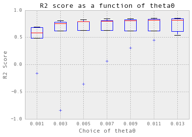
训练和测试每小时的数据
gp_hourlySteam, results_hourlySteam = predictAll(0.007, 0.01,
                                                 trainX_hourlySteam, trainY_hourlySteam,
                                                 testX_hourlySteam, testY_hourlySteam, testSet_hourlySteam, 'Hourly Steam (Particial)')
Train score R2: 0.844826486064
Test score R2: 0.570427290315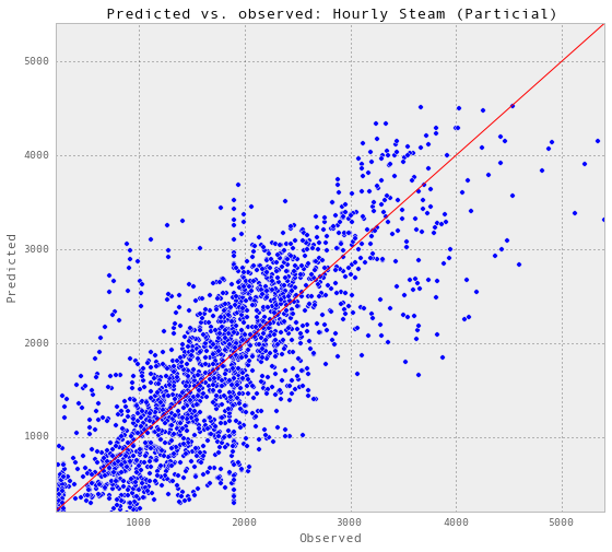
subset = results_hourlySteam['2014-01-26':'2014-02-01']
testY = subset['steam-LBS']
predictedY = subset['predictedY']
sigma = subset['sigma']

plotGP(testY, predictedY, sigma)

plt.ylabel('Steam (LBS)', fontsize = 13)
plt.title('Gaussian Process Regression: Hourly Steam Prediction', fontsize = 17)
plt.legend(loc='upper right')
plt.xlim([0, len(testY)])

xTickLabels = subset.index[np.arange(0,len(subset.index),6)]
ax = plt.gca()
ax.set_xticks(np.arange(0, len(subset), 6))
ax.set_xticklabels(labels = xTickLabels, fontsize = 13, rotation = 90)
plt.show()
以上是部分预测的可视化。
尝试训练和测试每小时的热水
警告:这可能需要很长时间才能执行代码。
# Warning: this could take forever to execute the code.

trainStart = '2012-01'
trainEnd = '2013-06'
testStart = '2013-07'
testEnd = '2014-10'

predictedElectricity = getPredictedElectricity(trainStart, trainEnd, testStart, testEnd)
# Steam
hourlySteamWithMoreFeatures = hourlySteamWithFeatures.join(predictedElectricity,
                                                           how = 'inner')

hourlySteamWithMoreFeatures = addHourlyTimeFeatures(hourlySteamWithMoreFeatures)

df_hourlySteam = hourlySteamWithMoreFeatures[['hour', 'cosHour', 'weekday',
                                              'day', 'week', 'occupancy', 'T-C',
                                              'humidityRatio-kg/kg',
                                              'predictedElectricity', 'steam-LBS']]

df = df_hourlySteam;

trainX_hourlySteam, trainY_hourlySteam, testX_hourlySteam, testY_hourlySteam, \
    testSet_hourlySteam = setTrainTestSets(df, trainStart, trainEnd,
                                           testStart, testEnd, 9)

gp_hourlySteam, results_hourlySteam = predictAll(0.007, 0.01,
                                                 trainX_hourlySteam, trainY_hourlySteam,
                                                 testX_hourlySteam, testY_hourlySteam,
                                                 testSet_hourlySteam)

results_hourlySteam.to_excel('Data/results_allHourlySteam.xlsx')
Final accuracy for hourly steam prediction.
results_allHourlySteam = pd.read_excel('Data/results_allHourlySteam.xlsx')

plotR2(results_allHourlySteam, 'steam-LBS', 'All Hourly Steam')
Test score R2: 0.84405417838
每小时的预测不如每天的好。但是R2的值仍然是0.85。
总结
高斯过程回归的整体性能非常好。GP的优点是提供了预测的不确定范围。缺点是对于大型数据集来说,它的计算开销非常大。