本文将介绍Gurobi中常用的两种数据结构:tuplelist和tupledict,并以案例文件中的网络流问题进行讲解
Gurobi的tuple类是Python中list的子类,tupledict是dict的子类。
在使用Gurobi建模时,推荐使用这两种类型,方便约束的编写,同时可以加快模型的读取速度。接下来将进行详细介绍:
本文主要参考了Gurobi 9.0.0目录中的refman.pdf
以下案例代码,不显式说明from gurobipy import *
tuplelist
构造函数
在构造函数中传入list对象可以将其转化为tuplelist类型
l = tuplelist(list)
例子:
l = tuplelist([(1,2),(1,3),(2,4)])
<gurobi.tuplelist (3 tuples, 2 values each):
 ( 1 , 2 )
 ( 1 , 3 )
 ( 2 , 4 )
筛选元素
select(pattern)函数返回一个根据pattern筛选的tuplelist对象。
> l = tuplelist([(1,2),(1,3),(2,4)])
<gurobi.tuplelist (3 tuples, 2 values each):
 ( 1 , 2 )
 ( 1 , 3 )
 ( 2 , 4 )
 > l.select() #返回所有的对象
<gurobi.tuplelist (3 tuples, 2 values each):
 ( 1 , 2 )
 ( 1 , 3 )
 ( 2 , 4 )
 # 可使用通配符
 > l.select(1,'*') # 返回第一位为1,第二为任意符号的元素
 <gurobi.tuplelist (2 tuples, 2 values each):
 ( 1 , 2 )
( 1 , 3 )tuplelist也可用in对其内部是否包含该元素进行判断(重写了__contains__())
> l = tuplelist([(1,2),(1,3),(2,4)])
<gurobi.tuplelist (3 tuples, 2 values each):
 ( 1 , 2 )
 ( 1 , 3 )
 ( 2 , 4 )
 # 判断是否有(1,2)
 if (1,2) in l:
    print("Tuple (1,2) is in tuplelist l")
tupledict
tupledict是Python类dict的子类,由键值两部分组成。key为上文提到的tuplelist,value为Gurobi的变量Var类型
tupledict可以方便地索引下标以及创建表达式
创建tupledict
构造函数
# 一个list,内部一个个元组,按照key,value先排好
dd = [((1,1),'a'), ((1,2),'b'),((2,1),'c'),((2,2),'d')]
# 相当于二元变量d_(i,j)
d = tupledict(dd)
{(1, 1): 'a', (1, 2): 'b', (2, 1): 'c', (2, 2): 'd'}
批量转换
multidict(data)函数提供将一个dict类型的对象data转化为tupledict。如果data的value包含了N个元素,则该函数返回的N+1个对象,第1个对象为data中的keys,后续对象为将N个value打散的tupledict。一次输入关于该元素的多组数据,并自动拆分为具有相同keys的
tupledictkeys, dict1, dict2 = multidict({'k1':[1,2], 'k2':[3,4], 'k3':[5,6]}) # 生成结果 # 原data中的键 tuplelist类型 keys = ['k1', 'k2', 'k3'] # 第一列元素 dict1 = {'k1': 1, 'k2': 3, 'k3': 5} # 第二列元素 dict2 = {'k1': 2, 'k2': 4, 'k3': 6}多元决策变量
在创建模型后,调用
addVars()函数,创建多维决策变量,该决策变量为tupledict类型m = Model() x = m.addVars(2,3) # 创建2*3的决策变量 # 使用下标方式进行访问 x[0,0] #<gurobi.Var C0>
筛选元素
- 与tuplelist相同,使用select()函数可以筛选出符合条件的key的value
- 像
dict一样,使用[]进行访问
d = tupledict([((1,1),'a'), ((1,2),'b'),((2,1),'c'),((2,2),'d')])
{(1, 1): 'a', (1, 2): 'b', (2, 1): 'c', (2, 2): 'd'}
# 显示所有元素
d.select()
# pattern筛选元素
d.select(1,'*')
['a', 'b']
# 下标访问
d[1,1]
'a'
集合运算(求和,连乘)
tupledict对象可进行求和sum(),乘积运算prod()。运算过后将会生成Gurobi内置的LinExpr()表达式对象,可作为约束添加至模型中。
sum(pattern)
pattern参数类似select的用法,可以为求和增加筛选条件
如果没有符合条件的pattern,则返回0
x = m.addVars(2,2)
expr = x.sum() # LinExpr: x[0,0] + x[0,1] + x[1,0] + x[1,1]
expr = x,sum(1, '*') # LinExpr: x[1,0] + x[1,1]

keys, dict1, dict2 = multidict({'k1':[1,2],
                                'k2':[3,4],
                                'k3':[5,6]})
dict1.sum() # LinExpr: 1 + 3 +5 = 9
prod(coeff,pattern)
coeff为一个dict类型,指定待计算的元素的系数。coeff的key要与待计算的集合中的key能对应
x = m.addVars(2,2)
coeff = {(0,0):1, (0,1):2,(1,0):3,(1,1):4}
expr = x.prod(coeff) # x[0,0] + 2*x[0,1] + 3*x[1,0] + 4*x[1,1]
expr = x.prod(coeff, 1,"*") # 3*x[1,0] + 4*x[1,1]
网络流案例详解
案例源文件根目录\example\python\netflow.py
该问题涉及到2种商品,2个发货地,3个收货地的配置问题,提供有各节点来往的成本,各地的最大库存量(流量)以及各节点的供、求关系,求满足供应条件的最小成本配置。
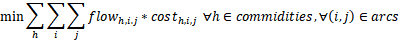
目标函数:
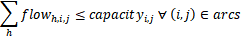
约束1:对于每种商品而言,不超过最大每个节点最大的容纳量
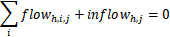
约束2:对于每种商品而言,满足每个节点的供应需求(本案例数据中,供给方为正,需求方为负)

将约束2拆开来看,则为:
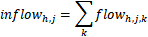
约束2.1 :供给方j的供应量=从j点流出的量
约束2.2:汇聚到需求方j的量+j点的需求(负数)=0
中文注释一下的代码粘贴如下:
#!/usr/bin/env python3.7

# Copyright 2019, Gurobi Optimization, LLC

# Solve a multi-commodity flow problem.  Two products ('Pencils' and 'Pens')
# are produced in 2 cities ('Detroit' and 'Denver') and must be sent to
# warehouses in 3 cities ('Boston', 'New York', and 'Seattle') to
# satisfy demand ('inflow[h,i]').
#
# Flows on the transportation network must respect arc capacity constraints
# ('capacity[i,j]'). The objective is to minimize the sum of the arc
# transportation costs ('cost[i,j]').

import gurobipy as gp
from gurobipy import GRB

# Base data
# 商品种类
commodities = ['Pencils', 'Pens']
# 所有的节点,作为key
nodes = ['Detroit', 'Denver', 'Boston', 'New York', 'Seattle']

arcs, capacity = gp.multidict({
    ('Detroit', 'Boston'):   100,
    ('Detroit', 'New York'):  80,
    ('Detroit', 'Seattle'):  120,
    ('Denver',  'Boston'):   120,
    ('Denver',  'New York'): 120,
    ('Denver',  'Seattle'):  120})
# arcs为tuplelist,表示节点间的连通关系
# capacity为tupledict,表示节点间的流量

# Cost for triplets commodity-source-destination
cost = {
    ('Pencils', 'Detroit', 'Boston'):   10,
    ('Pencils', 'Detroit', 'New York'): 20,
    ('Pencils', 'Detroit', 'Seattle'):  60,
    ('Pencils', 'Denver',  'Boston'):   40,
    ('Pencils', 'Denver',  'New York'): 40,
    ('Pencils', 'Denver',  'Seattle'):  30,
    ('Pens',    'Detroit', 'Boston'):   20,
    ('Pens',    'Detroit', 'New York'): 20,
    ('Pens',    'Detroit', 'Seattle'):  80,
    ('Pens',    'Denver',  'Boston'):   60,
    ('Pens',    'Denver',  'New York'): 70,
    ('Pens',    'Denver',  'Seattle'):  30}

# Demand for pairs of commodity-city
inflow = {
    ('Pencils', 'Detroit'):   50,
    ('Pencils', 'Denver'):    60,
    ('Pencils', 'Boston'):   -50,
    ('Pencils', 'New York'): -50,
    ('Pencils', 'Seattle'):  -10,
    ('Pens',    'Detroit'):   60,
    ('Pens',    'Denver'):    40,
    ('Pens',    'Boston'):   -40,
    ('Pens',    'New York'): -30,
    ('Pens',    'Seattle'):  -30}

# Create optimization model
m = gp.Model('netflow')

# Create variables
# 创建以commodities,arcs为下标的三维决策变量 flow_h,i,j
# obj=cost这种写法在创建变量时,设定好了目标函数
flow = m.addVars(commodities, arcs, obj=cost, name="flow")

# 添加约束1
# Arc-capacity constraints
m.addConstrs(
    (flow.sum('*', i, j) <= capacity[i, j] for i, j in arcs), "cap")

# 约束1的等价写法,将生成器改为for循环,逐个添加
# Equivalent version using Python looping
# for i, j in arcs:
#   m.addConstr(sum(flow[h, i, j] for h in commodities) <= capacity[i, j],
#               "cap[%s, %s]" % (i, j))

# 添加约束2
# Flow-conservation constraints
m.addConstrs(
    (flow.sum(h, '*', j) + inflow[h, j] == flow.sum(h, j, '*')
        for h in commodities for j in nodes), "node")

# 约束2的等价写法,将生成器改为for循环,逐个添加
# Alternate version:
# m.addConstrs(
#   (gp.quicksum(flow[h, i, j] for i, j in arcs.select('*', j)) + inflow[h, j] ==
#     gp.quicksum(flow[h, j, k] for j, k in arcs.select(j, '*'))
#     for h in commodities for j in nodes), "node")

# Compute optimal solution
m.optimize()

# Print solution
if m.status == GRB.OPTIMAL:
    solution = m.getAttr('x', flow)
    for h in commodities:
        print('\nOptimal flows for %s:' % h)
        for i, j in arcs:
            if solution[h, i, j] > 0:
                print('%s -> %s: %g' % (i, j, solution[h, i, j]))