caffe中卷积层反向传播原理

参考：https://blog.csdn.net/buyi_shizi/article/details/51512848，首先十分感谢该博主对caffe中反向传播原理的讲解，但是感觉该文章中对convlution layer的表述有问题。以下为本人的理解，如有错误还请批评指正

一、caffe卷积层反向传播代码实现

CAFFE_ROOT/src/caffe/layers/conv_layer.cpp

template <typename Dtype>
void ConvolutionLayer<Dtype>::Backward_cpu(const vector<Blob<Dtype>*>& top,
      const vector<bool>& propagate_down, const vector<Blob<Dtype>*>& bottom) {
  const Dtype* weight = this->blobs_[0]->cpu_data();
  Dtype* weight_diff = this->blobs_[0]->mutable_cpu_diff();
  for (int i = 0; i < top.size(); ++i) {
    const Dtype* top_diff = top[i]->cpu_diff();
    const Dtype* bottom_data = bottom[i]->cpu_data();
    Dtype* bottom_diff = bottom[i]->mutable_cpu_diff();
    // Bias gradient, if necessary.
    if (this->bias_term_ && this->param_propagate_down_[1]) {
      Dtype* bias_diff = this->blobs_[1]->mutable_cpu_diff();
      for (int n = 0; n < this->num_; ++n) {
        this->backward_cpu_bias(bias_diff, top_diff + n * this->top_dim_);
      }
    }
    if (this->param_propagate_down_[0] || propagate_down[i]) {
      for (int n = 0; n < this->num_; ++n) {
        // gradient w.r.t. weight. Note that we will accumulate diffs.
        if (this->param_propagate_down_[0]) {
          this->weight_cpu_gemm(bottom_data + n * this->bottom_dim_,
              top_diff + n * this->top_dim_, weight_diff);
        }
        // gradient w.r.t. bottom data, if necessary.
        if (propagate_down[i]) {
          this->backward_cpu_gemm(top_diff + n * this->top_dim_, weight,
              bottom_diff + n * this->bottom_dim_);
        }
      }
    }
  }
}

二、原理

batch-size为64

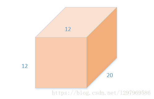
输入 input（12*12*20）
这里写图片描述

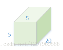
卷积核 weight（5*5*20）*50
这里写图片描述
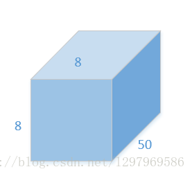
输出 output （8*8*50）

卷积操作存在权重和输入输出，反向传播需要计算总LOSS相对于该卷积层中输入、与权重的梯度Bottom diff与Weight diff（暂且不考虑偏置bias，原理是一样的）。输出的梯度Top diff为下一层的Bottom diff，反向传播中由下一层来提供。在该例子中，权重weight的参数个数为5*5*20*50。对于batch中的一个sample来说，需要进行的乘法操作数为（5*5*20）50（8*8），batch-size为64，则权重的总输入乘法为（5*5*20）50（8*8）*64，这时如果想一次求取所有对权值参数的梯度就比较困难，caffe中是逐样本对权值参数求梯度。然后再把所有的样本中的对于权值的梯度相加。对于单个样本：
这里写图片描述
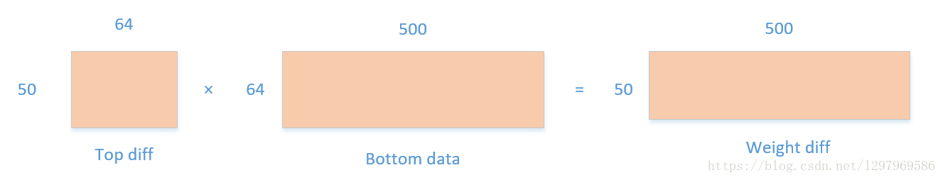
Top diff：为上一层的Bottom diff，尺寸为8*8*50，深度方向展开为二维50*64
△Bottom diff：为卷积核（5*5*20）在bottom-data上做滑动窗口操作时候对应的bottom-data的8*8个位置上的子块数据。展成二维为（5*5*20）*（8*8）=500*64大小。由BP算法的链式结构，以及在不考虑偏置bias的情况下WX=Y特性，权重梯度 Weight diff=Top diff*Bottom data。大小为500*50，对应卷积核参数（5*5*20）*50。当然这只是batch数据中的一个sample，在batch-size=64时，这个过程要经过64遍，然后把64个Weight diff相加后为最终Weight diff。

这里写图片描述
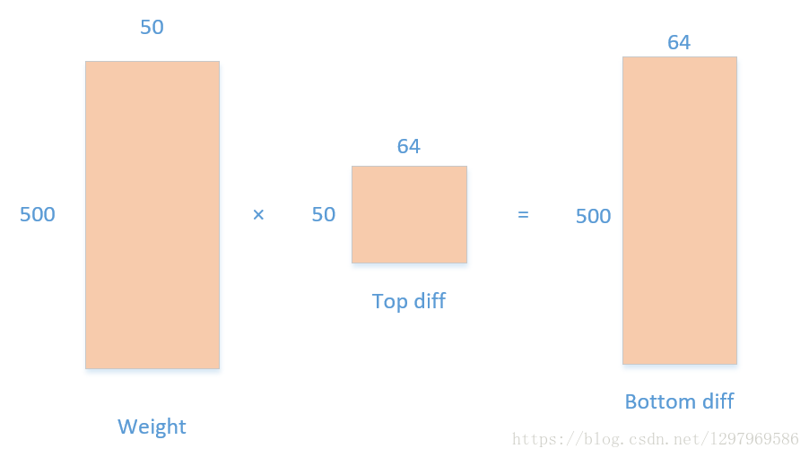
同理，在计算输入梯度时候，根据WX=Y，Bottom diff=Weight * Top diff ，其中Weight为（5*5*20）*50=500*50，
Top diff 为（8*8）*50=64*50。Bottom diff为500*64大小。这个500*64与12*12*20有什么联系呢？
其实，这个矩阵是对卷积核所遍历的64个5*5*20个子块的梯度。