Softmax Regression
The Logistic Regression model can be generalized to support multiple classes directly, without having to train and combine multiple binary classifiers (as discussed in https://blog.csdn.net/Linli522362242/article/details/103786116). This is called Softmax Regression, or Multinomial Logistic Regression.
The idea is quite simple: when given an instance x, the Softmax Regression model first computes a score ![]() for each class k, then estimates the probability of each class by applying the softmax function (also called the normalized exponential) to the scores. The equation to compute
for each class k, then estimates the probability of each class by applying the softmax function (also called the normalized exponential) to the scores. The equation to compute ![]() should look familiar, as it is just like the equation for Linear Regression prediction (see Equation 4-19).
should look familiar, as it is just like the equation for Linear Regression prediction (see Equation 4-19).
Equation 4-19. Softmax score for class k ![]()
Note that each class has its own dedicated parameter vector ![]() . All these vectors are typically stored as rows in a parameter matrix
. All these vectors are typically stored as rows in a parameter matrix ![]() . Note
. Note ![]() ==b
==b
[ #class0, class1, ...., classN
[b0==1, b0==1, ... repeat...],
[b1, b1, ..., repeat...],
... ...
[bk, bk, ... repeat...]
]
Theta: (number_of_theta=features plus the bias term , number of label names/class )![]() : (number of label names/class , number_of_theta
: (number of label names/class , number_of_theta![]() =features plus the bias term )
=features plus the bias term )
X_train( number of features plus the bias term, number of instances): one column is a instance,
[ [x_b0==1, x_b0==1, ... repeat...], [x_b1, x_b1, ... repeat...], ..., [x_bk, x_bk, ... repeat...]]
logits = ![]() :
: ![]() ; p is corresponding to features including bias/intercept
; p is corresponding to features including bias/intercept
Once you have computed the score of every class for the instance x, you can estimate the probability ![]() that the instance belongs to class k by running the scores through the softmax function (Equation 4-20): it computes the exponential of every score, then normalizes them (dividing by the sum of all the exponentials).
that the instance belongs to class k by running the scores through the softmax function (Equation 4-20): it computes the exponential of every score, then normalizes them (dividing by the sum of all the exponentials).
Equation 4-20. Softmax function 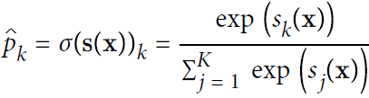
• K is the number of classes.
• s(x) is a vector containing the scores of each class for the instance x.
•![]() is the estimated probability that the instance x belongs to class k given the scores of each class for that instance.
is the estimated probability that the instance x belongs to class k given the scores of each class for that instance.
Just like the Logistic Regression classifier, the Softmax Regression classifier predicts the class with the highest estimated probability (which is simply the class with the highest score), as shown in Equation 4-21.
Equation 4-21. Softmax Regression classifier prediction ![]()
The argmax operator returns the value of a variable that maximizes a function. In this equation, it returns the value of k that maximizes the estimated probability ![]() .
.
return index/k max of ==> return index/k max of ![]()
##########################################
TIP
The Softmax Regression classifier predicts only one class at a time (i.e., it is multiclass, not multioutput) so it should be used only with mutually exclusive classes such as different types of plants. You cannot use it to recognize multiple people in one picture.
##########################################
Now that you know how the model estimates probabilities and makes predictions, let’s take a look at training. The objective is to have a model that estimates a high probability for the target class (and consequently a low probability for the other classes). Minimizing the cost function shown in Equation 4-22, called the cross entropy交叉熵, should lead to this objective because it penalizes the model when it estimates a low probability for a target class. Cross entropy is frequently used to measure how well a set of estimated class probabilities match the target classes.
Equation 4-22. Cross entropy cost function 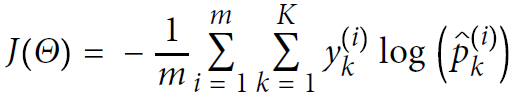
![]() is equal to 1 if the target class for the ith instance is k; otherwise, it is equal to 0.
is equal to 1 if the target class for the ith instance is k; otherwise, it is equal to 0.
Notice that when there are just two classes (K = 2), this cost function is equivalent to the Logistic Regression’s cost function (log loss; see Equation 4-17 ![]() ).
).
############################################################################
CROSS ENTROPY
Cross entropy originated from information theory. Suppose you want to efficiently transmit information about the weather every day. If there are eight options (sunny, rainy, etc.), you could encode each option using 3 bits since ![]() = 8. However, if you think it will be sunny almost every day, it would be much more efficient to code “sunny” on just one bit (0_ _ _) and the other seven options on 4 bits (starting with a 1 _ _ _). Cross entropy measures the average number of bits you actually send per option. If your assumption about the weather is perfect, cross entropy will just be equal to the entropy of the weather itself (i.e., its intrinsic unpredictability内在的不可预测性). But if your assumptions are wrong (e.g., if it rains often), cross entropy will be greater by an amount called the Kullback–Leibler divergence.
= 8. However, if you think it will be sunny almost every day, it would be much more efficient to code “sunny” on just one bit (0_ _ _) and the other seven options on 4 bits (starting with a 1 _ _ _). Cross entropy measures the average number of bits you actually send per option. If your assumption about the weather is perfect, cross entropy will just be equal to the entropy of the weather itself (i.e., its intrinsic unpredictability内在的不可预测性). But if your assumptions are wrong (e.g., if it rains often), cross entropy will be greater by an amount called the Kullback–Leibler divergence.
The cross entropy between two probability distributions p and q is defined as ![]() (at least when the distributions are discrete).
(at least when the distributions are discrete).
###################################extra materials
Classification Trees
Recall that for a regression tree, the predicted response(y) for an observation(one instance) is given by the mean response of the training observations that belong to the same terminal node. ![]()
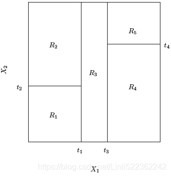
for a classification tree, we predict that each observation belongs to the most commonly occurring class最常
出现的类 of training observations in the region(Prediction via Stratification of the Feature Space: We divide the predictor space—that is, the set of possible values for X1,X2, . . .,Xp—into J distinct and non-overlapping regions, R1,R2, . . . , RJ ) to which it belongs. In interpreting the results of a classification tree, we are often interested not only in the class prediction corresponding to a particular terminal node region, but also in the class proportions among the training observations that fall into that region
in the classification setting, RSS cannot be used as a criterion for making the binary splits. A natural alternative to RSS is the classification error rate. Since we plan classification to assign an observation in a given region to the most commonly occurring error rate class of training observations in that region, the classification error rate is simply the fraction of the training observations in that region that do not belong to the most common class:![]()
Here ˆpmk represents the proportion of training observations(instances) in the mth region that are from the kth class(e.g. Iris virginica, Iris versicolor, Iris setosa). However, it turns out that classification error is not sufficiently sensitive for tree-growing, and in practice two other measures are preferable.
######################
If X ~ B(n, p), that is, X is a binomially distributed random variable, n being the total number of experiments and p the probability of each experiment yielding a successful result, then the expected value of X is: ![]()
This follows from the linearity of the expected value along with fact that X is the sum of n identical Bernoulli random variables, each with expected value p. In other words, if ![]() are identical (and independent) Bernoulli random variables with parameter p, then
are identical (and independent) Bernoulli random variables with parameter p, then ![]() and
and ![]()
The variance is: ![]()
######################
The Gini index is defined by 
a measure of total variance across the K classes. It is not hard to see that the Gini index takes on a small value
(p=0.9, K * p *q= K*0.9*0.1== 0.09*K) if all of the ˆpmk’s are close to zero or one. For this reason the Gini index is referred to as a measure of node purity—a small value indicates that a node contains predominantly显著地 observations from a single class.
An alternative to the Gini index is cross-entropy, given by 
Since 0 ≤ ˆpmk ≤ 1, it follows that 0 ≤ − ˆpmk* logˆpmk. One can show that the cross-entropy will take on a value near zero if the ˆpmk’s are all near zero or near one(e.g. ˆpmk=0.1, -K*0.1*(log0.1)==0.1*K). Therefore, like the Gini index, the cross-entropy will take on a small value if the mth node is pure. In fact, it turns out that the Gini index and the cross-entropy are quite similar numerically.
############################################################################
Equation 4-23. Cross entropy gradient vector for class k 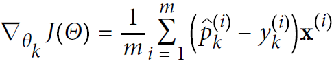
Now you can compute the gradient vector for every class, then use Gradient Descent (or any other optimization algorithm) to find the parameter matrix Θ that minimizes the cost function.![]() # [[pk0 - yk0, pk1-yk1, pk2-yk2], [pk0 - yk0, pk1-yk1, pk2-yk2],...,]
# [[pk0 - yk0, pk1-yk1, pk2-yk2], [pk0 - yk0, pk1-yk1, pk2-yk2],...,]
#each row is corresponding to an instance, each column is a class/label
Let’s use Softmax Regression to classify the iris flowers into all three classes. Scikit-Learn’s LogisticRegression uses one-versus-all by default when you train it on more than two classes, but you can set the multi_class hyperparameter to "multinomial" to switch it to Softmax Regression instead. You must also specify a solver that supports
Softmax Regression, such as the "lbfgs" solver (see Scikit-Learn’s documentation for more details https://scikit-learn.org/stable/modules/generated/sklearn.linear_model.LogisticRegression.html). It also applies ℓ2 regularization by default, which you can control using the hyperparameter C.
class sklearn.linear_model.LogisticRegression(penalty='l2', dual=False, tol=0.0001, C=1.0, fit_intercept=True, intercept_scaling=1, class_weight=None, random_state=None, solver='lbfgs', max_iter=100, multi_class='auto', verbose=0, warm_start=False, n_jobs=None, l1_ratio=None)
In the multiclass case, the training algorithm uses the one-vs-rest (OvR) scheme if the ‘multi_class’ option is set to ‘ovr’, and uses the cross-entropy loss if the ‘multi_class’ option is set to ‘multinomial’. (Currently the ‘multinomial’ option is supported only by the ‘lbfgs’, ‘sag’, ‘saga’ and ‘newton-cg’ solvers.)
C: float, default=1.0
Inverse of regularization strength; must be a positive float. Like in support vector machines, smaller values specify stronger regularization.
multi_class{‘auto’, ‘ovr’, ‘multinomial’}, default=’auto’
If the option chosen is ‘ovr’, then a binary problem is fit for each label. For ‘multinomial’ the loss minimised is the multinomial loss fit across the entire probability distribution, even when the data is binary. ‘multinomial’ is unavailable when solver=’liblinear’. ‘auto’ selects ‘ovr’ if the data is binary, or if solver=’liblinear’, and otherwise selects ‘multinomial’.
X = iris["data"][:, (2,3)] # petal length, petal width
y = iris["target"]

softmax_reg = LogisticRegression(multi_class="multinomial", solver="lbfgs", C=10, random_state=42)
softmax_reg.fit(X,y)softmax_reg.predict([[5,2],])![]()
softmax_reg.predict_proba([[5,2],])![]()

So the next time you find an iris with 5 cm long and 2 cm wide petals, you can ask your model to tell you what type of iris it is, and it will answer Iris-Virginica (class 2) with 94.2% probability (or Iris-Versicolor with 5.8% probability)
Figure 4-25 shows the resulting decision boundaries, represented by the background colors. Notice that the decision boundaries between any two classes are linear. The figure also shows the probabilities for the Iris-Versicolor class, represented by the curved lines (e.g., the line labeled with 0.450 represents the 45% probability boundary).
Notice that the model can predict a class that has an estimated probability below 50%. For example, at the point where all decision boundaries meet, all classes have an equal estimated probability of 33% ![]() .
.
x0, x1 = np.meshgrid(
    np.linspace(0,8, 500).reshape(-1,1), #[[500 rows] 1 column]
    np.linspace(0,3.5, 200).reshape(-1,1), #[[200 rows] 1 column]
)
#x0: [[0,...500 columns...,8]...200 rows...[0,...500...,8]]
#x1: [[0...500 columns...,0]...200 rows...[3.5,...500...,3.5]]
X_new = np.c_[x0.ravel(), x1.ravel()] ##[100000=200*500, 200*500]

y_proba = softmax_reg.predict_proba(X_new) #[[Iris-Setosa,Iris-Versicolour,Iris-Virginica], ...100000 rows...[Iris-Setosa,Iris-Versicolour,Iris-Virginica]]
y_predict = softmax_reg.predict(X_new) #[class 0,class2,class1,...] 100 000 elements

zz1 = y_proba[:,1].reshape(x0.shape) #Iris-Versicolour
zz = y_predict.reshape(x0.shape)

plt.figure(figsize=(10,4))
plt.plot(X[y==2, 0], X[y==2, 1], "g^", label="Iris virginica")
plt.plot(X[y==1, 0], X[y==1, 1], "bs", label="Iris versicolor")
plt.plot(X[y==0, 0], X[y==0, 1], "yo", label="Iris setosa")
points=np.array([[5,2],])
plt.plot(points[:,0], points[:,1], "ko",markersize=10, label="an iris(5 cm, 2 cm)")

from matplotlib.colors import ListedColormap
custom_cmap = ListedColormap(['#fafab0','#9898ff','#a0faa0'])

plt.contourf(x0, x1, zz, cmap=custom_cmap) # y_predict value on contour
contour = plt.contour(x0, x1, zz1, cmap=plt.cm.brg) #y_proba belong to Iris-Versicolour on boundaries
plt.clabel(contour, inline=True, fontsize=12)
plt.xlabel("Petal length", fontsize=14)
plt.ylabel("Petal width", fontsize=14)
plt.legend(loc="center left", fontsize=14)
plt.axis([0,7,0,3.5])
plt.title("Figure 4-25. Softmax Regression decision boundaries")
plt.show()
Exercises
1. What Linear Regression training algorithm can you use if you have a training set with millions of features?
Ans: If you have a training set with millions of features you can use Stochastic Gradient Descent or Minibatch Gradient Descent, and perhaps Batch Gradient Descent if the training set fits in memory. But you cannot use the Normal Equation![]() because the computational complexity(
because the computational complexity(![]() , where n is the number of features) grows quickly (more than quadratically) with the number of features.
, where n is the number of features) grows quickly (more than quadratically) with the number of features.
2. Suppose the features in your training set have very different scales. What algorithms might suffer from this, and how? What can you do about it?https://blog.csdn.net/Linli522362242/article/details/104005906
Ans: If the features in your training set have very different scales, the cost function will have the shape of an elongated bowl, so the Gradient Descent algorithms will take a long time to converge. To solve this you should scale the data before training the model. Note that the Normal Equation will work just fine without scaling. Moreover, regularized models may converge to a suboptimal solution if the features are not scaled: indeed, since regularization penalizes large weights, features with smaller values will tend to be ignored compared to features with larger values.
3. Can Gradient Descent get stuck in a local minimum when training a Logistic Regression model?
Ans: Gradient Descent cannot get stuck in a local minimum when training a Logistic Regression model because the cost function is convex. https://blog.csdn.net/Linli522362242/article/details/104070847

4. Do all Gradient Descent algorithms lead to the same model provided(相同的模型参数) you let them run long enough?
Ans: If the optimization problem is convex (such as Linear Regression or Logistic Regression), and assuming the learning rate is not too high, then all Gradient Descent algorithms will approach the global optimum and end up producing fairly similar models. However, unless you gradually reduce the learning rate, Stochastic GD and Mini-batch GD will never truly converge; instead, they will keep jumping back and forth around the global optimum. This means that even if you let them run for a very long time, these Gradient Descent algorithms will produce slightly different models.
5. Suppose you use Batch Gradient Descent and you plot the validation error at every epoch. If you notice that the validation error consistently goes up, what is likely going on? How can you fix this?
Ans: If the validation error consistently goes up after every epoch, then one possibility is that the learning rate is too high and the algorithm is diverging. If the training error also goes up, then this is clearly the problem and you should reduce the learning rate. However, if the training error is not going up, then your model is overfitting the training set and you should stop training.
6. Is it a good idea to stop Mini-batch Gradient Descent immediately when the validation error goes up?
Ans: Due to their random nature, neither Stochastic Gradient Descent nor Mini-batch Gradient Descent is guaranteed to make progress at every single training iteration. So if you immediately stop training when the validation error goes up, you may stop much too early, before the optimum is reached. A better option is to save the model at regular intervals, and when it has not improved for a long time (meaning it will probably never beat the record), you can revert to the best saved model.
7. Which Gradient Descent algorithm (among those we discussed) will reach the vicinity附近 of the optimal solution the fastest? Which will actually converge? How can you make the others converge as well?
Ans: Stochastic Gradient Descent has the fastest training iteration since it considers only one training instance at a time, so it is generally the first to reach the vicinity of the global optimum (or Minibatch GD with a very small mini-batch size). However, only Batch Gradient Descent will actually converge, given enough training time. As mentioned, Stochastic GD and Mini-batch GD will bounce around the optimum, unless you gradually reduce the learning rate.
8. Suppose you are using Polynomial Regression. You plot the learning curves and you notice that there is a large gap between the training error and the validation error. What is happening? What are three ways to solve this?
 https://blog.csdn.net/Linli522362242/article/details/104097191
Ans: If the validation error is much higher than the training error, this is likely because your model is overfitting the training set. One way to try to fix this is to reduce the polynomial degree: a model with fewer degrees of freedom is less likely to overfit. Another thing you can try is to regularize the model — for example, by adding an ℓ2 penalty (Ridge) or an ℓ1 penalty (Lasso) to the cost function. This will also reduce the degrees of freedom of the model. Lastly, you can try to increase the size of the training set.
9. Suppose you are using Ridge Regression and you notice that the training error and the validation error are almost equal and fairly high. Would you say that the model suffers from high bias or high variance? Should you increase the regularization hyperparameter α or reduce it?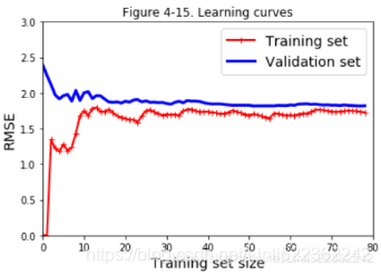
Ans: If both the training error and the validation error are almost equal and fairly high, the model is likely underfitting the training set, which means it has a high bias. You should try reducing the regularization hyperparameter α.
10. Why would you want to use:
• Ridge Regression instead of Linear Regression?
• Lasso instead of Ridge Regression?
• Elastic Net instead of Lasso?
Ans: Let’s see:
A model with some regularization typically performs better than a model without any regularization, so you should generally prefer Ridge Regression over plain Linear Regression.2 Lasso Regression uses an ℓ1 penalty, which tends to push the weights down to exactly zero. This leads to sparse models, where all weights are zero except for the most important weights. This is a way to perform feature selection automatically, which is good if you suspect that only
a few features actually matter. When you are not sure, you should prefer Ridge Regression. Elastic Net is generally preferred over Lasso since Lasso may behave erratically in some cases (when several features are strongly correlated or when there are more features(PolynomialFeatures(degree=d) ) than training instances). However, it does add an extra hyperparameter to tune. If you just want Lasso without the erratic behavior, you can just use Elastic Net with an l1_ratio close to 1.
11. Suppose you want to classify pictures as outdoor/indoor and daytime/nighttime. Should you implement two Logistic Regression classifiers or one Softmax Regression classifier?
Ans: If you want to classify pictures as outdoor/indoor and daytime/nighttime, since these are not exclusive classes (i.e., all four combinations are possible) you should train two Logistic Regression classifiers.
12. Implement Batch Gradient Descent with early stopping for Softmax Regression (without using Scikit-Learn).
Ans: (without using Scikit-Learn) Let's start by loading the data. We will just reuse the Iris dataset we loaded earlier.
X = iris["data"][:, (2,3)] #petal length, petal width
y = iris["target"]
X[:5]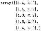
We need to add the bias term for every instance (X0 =1):
X_with_bias = np.c_[ np.ones([len(X), 1]), X ] #[[x_b0==1 , x_b1 , x_b2 ], ...repeat]
X_with_bias[:5]
And let's set the random seed so the output of this exercise solution is reproducible:
np.random.seed(2042)The easiest option to split the dataset into a training set, a validation set and a test set would be to use Scikit Learn's train_test_split() function, but the point of this exercise is to try understand the algorithms by implementing them manually. So here is one possible implementation:
test_ratio = 0.2
validation_ratio = 0.2
total_size = len(X_with_bias)

test_size = int(total_size*validation_ratio)
validation_size = int(total_size*validation_ratio)
train_size = total_size - test_size - validation_size

rnd_indices = np.random.permutation(total_size) #Shuffle

X_train = X_with_bias[rnd_indices[:train_size]]
y_train = y[rnd_indices[:train_size]]
X_valid = X_with_bias[rnd_indices[train_size:-test_size]]
y_valid = y[rnd_indices[train_size:-test_size]]
X_test = X_with_bias[rnd_indices[-test_size:]]
y_test = y[rnd_indices[-test_size:]]
The targets are currently class indices (0, 1 or 2), but we need target class probabilities to train the Softmax Regression model. Each instance will have target class probabilities equal to 0.0 for all classes except for the target class which will have a probability of 1.0 (in other words, the vector of class probabilities for a given instance is a one-hot vector). Let's write a small function to convert the vector of class indices into a matrix containing a one-hot vector for each instance:
#each row is a instance, the corresponding target class/label will decide
#which cell will be assigned with 1 and the rest will be set with 0
def to_one_hot(y):
    n_classes = len(set(y))#y.max() + 1
    m = len(y)
    Y_one_hot = np.zeros( (m,n_classes) ) #(number of instance, number of label names)
    Y_one_hot[np.arange(m),y]=1 #base on list(set(y))=[0,1,2]
    return Y_one_hot
Let's test this function on the first 10 instances:
y_train[:10]![]()
to_one_hot(y_train[:10])
Looks good, so let's create the target class probabilities matrix for the training set and the test set:
Y_train_one_hot = to_one_hot(y_train)
Y_valid_one_hot = to_one_hot(y_valid)
Y_test_one_hot = to_one_hot(y_test)
Now let's implement the Softmax function. Recall that it is defined by the following equation: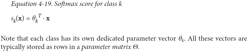
X_train: [ [x_b0==1 , x_b1 , x_b2 ], ...repeat..., [x_b0==1 , x_b1 , x_b2 ]] #each row is an instance
Theta: (number_of_theta=features plus the bias term, number of label names/ class)
logits = X_train.dot(Theta) : ![]()

def softmax(logits):
    exps = np.exp(logits)
    exp_sums = np.sum(exps, axis=1, keepdims=True)
    return exps / exp_sums # each row has different theta_i in different class_k
We are almost ready to start training. Let's define the number of inputs and outputs:
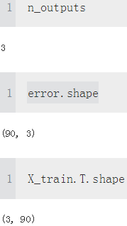
n_inputs = X_train.shape[1] # == 3 (2 features plus the bias term)
n_outputs = len(np.unique(y_train)) # == 3 (3 iris classes)
Now here comes the hardest part: training! Theoretically, it's simple: it's just a matter of translating the math equations into Python code. But in practice, it can be quite tricky: in particular, it's easy to mix up the order of the terms, or the indices. You can even end up with code that looks like it's working but is actually not computing exactly the right thing. When unsure, you should write down the shape of each term in the equation and make sure the corresponding terms in your code match closely. It can also help to evaluate each term independently and print them out. The good news it that you won't have to do this everyday, since all this is well implemented by Scikit-Learn, but it will help you understand what's going on under the hood.
So the equations we will need are the cost function:
![]() : np.sum(Y_train_one_hot * np.log(Y_proba+epsilon), axis=1)
: np.sum(Y_train_one_hot * np.log(Y_proba+epsilon), axis=1)![]() : loss = -np.mean( np.sum(Y_train_one_hot * np.log(Y_proba+epsilon), axis=1) )
: loss = -np.mean( np.sum(Y_train_one_hot * np.log(Y_proba+epsilon), axis=1) )
And the equation for the gradients:
Note that ![]() may not be computable if
may not be computable if ![]() . So we will add a tiny value
. So we will add a tiny value ![]() to
to ![]() to avoid getting
to avoid getting nan values.
logits = X_train.dot(Theta)
logits = X_valid.dot(Theta)
eta = 0.01
n_iterations = 5001
epsilon = 1e-7
                        #(3==2 features plus the bias term, 3 iris classes)
Theta = np.random.randn(n_inputs, n_outputs) #(theta group, 3 labels)

for iteration in range(n_iterations):
    logits = X_train.dot(Theta) #softmax score
    Y_proba = softmax(logits) #softmax function              #epsion is a noise
    loss = -np.mean( np.sum(Y_train_one_hot * np.log(Y_proba+epsilon), axis=1) ) #Cross entropy cost function
    #np.sum(Y_train_one_hot * np.log(Y_proba+epsilon), axis=1) # Cross entropy
    error = Y_proba - Y_train_one_hot # [[pk0 - yk0, pk1-yk1, pk2-yk2],...,]
                                      #each row is corresponding to an instance, each column is a class/label
    if iteration % 500 == 0: #sampling
        print(iteration, loss)     #X_train.T: [ [x_b0==1 , x_b0==1 ,..., x_b0==1 ], [x_b1,x_b1,...,x_b1], [x_b2 , x_b2 ,..., x_b2 ]]   #each column is an instance
    gradients = 1/m * X_train.T.dot(error) # Cross entropy gradient vector
    Theta = Theta - eta*gradients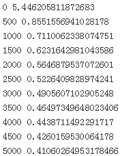
And that's it! The Softmax model is trained. Let's look at the model parameters:
Theta # (number_of_theta=features plus the bias term, number of label names/ class) # parameter matrix Θ
Let's make predictions for the validation set and check the accuracy score: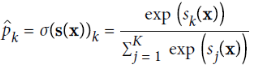

logits = X_valid.dot(Theta) #X_valid:[ [x_b0==1 , x_b1 , x_b2 ], ...repeat..., [x_b0==1 , x_b1 , x_b2 ]]#each row is an instance
Y_proba = softmax(logits) #Softmax function #the estimated probability
y_predict = np.argmax(Y_proba,axis=1) #get each instance' predicted class/label
y_predict ![]()
accuracy_score = np.mean(y_predict==y_valid)
accuracy_score![]()
Well, this model looks pretty good. For the sake of the exercise, let's add a bit of ![]() ==
==  regularization. The following training code is similar to the one above, but the loss now has an additional
 ![]() penalty, and the gradients have the proper additional term (note that we don't regularize the first element of
penalty, and the gradients have the proper additional term (note that we don't regularize the first element of Theta since this corresponds to the bias term). Also, let's try increasing the learning rate eta.
(Note: usually we are not using the term ![]() , but here we use it since the author's idea)
, but here we use it since the author's idea)
#Cross entropy cost function +
+
Then Cross entropy gradient vector for class k
 +
+ ![]()
![]()
eta = 0.1 ##########
n_iterations = 5001
epsilon = 1e-7
m = len(X_train)
alpha = 0.1 #  regularization hyperparameter
                        ##(3==2 features plus the bias term, 3 iris classes)
Theta = np.random.randn(n_inputs, n_outputs) #(theta, 3 labels)

for iteration in range(n_iterations):
    logits = X_train.dot(Theta) #softmax score
    Y_proba = softmax(logits)  #softmax function
    #Cross entropy cost function                                      #epsion is a noise
    xentropy_loss = -np.mean( np.sum(Y_train_one_hot * np.log(Y_proba+epsilon), axis=1) )
    l2_loss = 1/2 * np.sum(np.square(Theta[1:]))
    loss = xentropy_loss + alpha * l2_loss

    error = Y_proba - Y_train_one_hot # [[pk0 - yk0, pk1-yk1, pk2-yk2],...,]
                                      #each row is corresponding to an instance, each column is a class/label
    if iteration % 500 == 0: #sampling
        print(iteration, loss)  ##X_train.T: [ [x_b0==1 , x_b0==1 ,..., x_b0==1 ], [x_b1,x_b1,...,x_b1], [x_b2 , x_b2 ,..., x_b2 ]]   #each column is an instance
    gradients = 1/m * X_train.T.dot(error) + np.r_[ np.zeros((1, n_outputs)), alpha*Theta[1:] ]# Cross entropy gradient vector
    Theta = Theta - eta*gradients
Because of the additional ![]() penalty, the loss seems greater than earlier, but perhaps this model will perform better? Let's find out:
penalty, the loss seems greater than earlier, but perhaps this model will perform better? Let's find out:
logits = X_valid.dot(Theta)
Y_proba = softmax(logits)
y_predict = np.argmax(Y_proba,axis=1)

accuracy_score = np.mean(y_predict == y_valid)
accuracy_score
Cool, perfect accuracy! We probably just got lucky with this validation set, but still, it's pleasant.
Now let's add early stopping(since the cost function is convex). For this we just need to measure the loss on the validation set at every iteration and stop when the error starts growing.
eta = 0.1 ##########
n_iterations = 5001
epsilon = 1e-7
m = len(X_train)
alpha = 0.1 #  regularization hyperparameter
best_loss = np.infty###########
                        ##(3==2 features plus the bias term, 3 iris classes)
Theta = np.random.randn(n_inputs, n_outputs) #(theta, 3 labels)

for iteration in range(n_iterations):
    logits = X_train.dot(Theta) #softmax score
    Y_proba = softmax(logits)  #softmax function
    #Cross entropy cost function                                      #epsion is a noise
    xentropy_loss = -np.mean( np.sum(Y_train_one_hot * np.log(Y_proba+epsilon), axis=1) )
    l2_loss = 1/2 * np.sum(np.square(Theta[1:]))
    loss = xentropy_loss + alpha * l2_loss

    error = Y_proba - Y_train_one_hot # [[pk0 - yk0, pk1-yk1, pk2-yk2],...,]
                                      #each row is corresponding to an instance, each column is a class/label
    gradients = 1/m * X_train.T.dot(error) + np.r_[ np.zeros((1, n_outputs)), alpha*Theta[1:] ]# Cross entropy gradient vector
    Theta = Theta - eta*gradients

    logits = X_valid.dot(Theta) #prediction #softmax score
    Y_proba = softmax(logits) #softmax function
    xentropy_loss = -np.mean( np.sum(Y_valid_one_hot * np.log(Y_proba+epsilon), axis=1) ) #Cross entropy cost function
    l2_loss = 1/2 * np.sum( np.square(Theta[1:]))
    loss = xentropy_loss + alpha*l2_loss

    if iteration % 500 == 0: #sampling
        print(iteration, loss)  ##X_train.T: [ [x_b0==1 , x_b0==1 ,..., x_b0==1 ], [x_b1,x_b1,...,x_b1], [x_b2 , x_b2 ,..., x_b2 ]]   #each column is an instance

    if loss<best_loss:
        best_loss = loss
    else:
        print(iteration-1, best_loss)
        print(iteration, loss, "early stopping")
        break
logits = X_valid.dot(Theta)
Y_proba = softmax(logits)
y_predict = np.argmax(Y_proba, axis=1)
accuracy_score = np.mean(y_predict == y_valid)
accuracy_score![]()
Still perfect, but faster.
Now let's plot the model's predictions on the whole dataset:
x0, x1 = np.meshgrid(
    np.linspace(0,8, 500).reshape(-1,1),#[[500 rows] 1 column]
    np.linspace(0,3.5, 200).reshape(-1,1),#[[200 rows] 1 column]
)
#x0: [[0,...500 columns...,8]...200 rows...[0,...500...,8]]
#x1: [[0...500 columns...,0]...200 rows...[3.5,...500...,3.5]]
X_new = np.c_[x0.ravel(), x1.ravel()] #[100000=200*500, 200*500]
X_new_with_bias = np.c_[np.ones((len(X_new),1)), X_new]

logits = X_new_with_bias.dot(Theta)#[[Iris-Setosa,Iris-Versicolour,Iris-Virginica], ...[Iris-Setosa,Iris-Versicolour,Iris-Virginica]]
Y_proba = softmax(logits)
y_predict = np.argmax(Y_proba, axis=1) #[class 0,class2,class1,...for each row/instance...]

zz1 = Y_proba[:,1].reshape(x0.shape)#Iris-Versicolour
zz = y_predict.reshape(x0.shape)

plt.figure(figsize=(10,4))
plt.plot(X[y==2, 0], X[y==2,1], "g^", label="Iris virginica")
plt.plot(X[y==1, 0], X[y==1,1], "bs", label="Iris versicolor")
plt.plot(X[y==0, 0], X[y==0,1], "yo", label="Iris setosa")

from matplotlib.colors import ListedColormap
custom_cmap = ListedColormap(['#fafab0','#9898ff','#a0faa0'])

plt.contourf(x0, x1, zz, cmap=custom_cmap)
contour= plt.contour(x0, x1, zz1, cmap=plt.cm.brg)
plt.clabel(contour, inline=1, fontsize=12)
plt.xlabel("Petal length", fontsize=14)
plt.ylabel("Petal width", fontsize=14)
plt.legend(loc="upper left", fontsize=14)
plt.axis([0,7, 0,3.5])
plt.show()
And now let's measure the final model's accuracy on the test set:
logits = X_test.dot(Theta)
Y_proba = softmax(logits)
y_predict = np.argmax(Y_proba, axis=1)

accuracy_score = np.mean(y_predict==y_test)
accuracy_score![]()
![]()
Our perfect model turns out to have slight imperfections. This variability is likely due to the very small size of the dataset: depending on how you sample the training set, validation set and the test set, you can get quite different results. Try changing the random seed and running the code again a few times, you will see that the results will vary.
