04_TrainingModels_Normal Equation(正态方程,正规方程) Derivation_Gradient Descent_Polynomial Regression

So far we have treated Machine Learning models and their training algorithms mostly like black boxes. If you went through some of the exercises in the previous, you may have been surprised by how much you can get done without knowing anything about what’s under the hood幕后: you optimized a regression system, you improved a digit image classifier, and you even built a spam classifier from scratch — all this without knowing how they actually work. Indeed, in many situations you don’t really need to know the implementation details.

However, having a good understanding of how things work can help you quickly home找到 in on the appropriate model, the right training algorithm to use, and a good set of hyperparameters for your task. Understanding what’s under the hood黑箱子内部 will also help you debug issues and perform error analysis more efficiently. Lastly, most of the topics discussed in this chapter will be essential in understanding, building, and training neural networks (discussed in Part II of this book).

In this chapter, we will start by looking at the Linear Regression model, one of the simplest models there is. We will discuss two very different ways to train it:

• Using a direct “closed-form” equation that directly computes the model parameters that best fit the model to the training set (i.e., the model parameters that minimize the cost function over the training set).
• Using an iterative optimization approach, called Gradient Descent梯度下降 (GD), that gradually tweaks the model parameters to minimize the cost function over the training set, eventually converging收敛 to the same set of parameters as the first method. We will look at a few variants of Gradient Descent that we will use again and again when we study neural networks in Part II: Batch GD, Mini-batch GD, and Stochastic GD.

Next we will look at Polynomial Regression多项式回归, a more complex model that can fit nonlinear datasets. Since this model has more parameters than Linear Regression, it is more prone to更容易 overfitting the training data, so we will look at how to detect whether or not this is the case, using learning curves, and then we will look at several regularization正则化 techniques that can reduce the risk of overfitting the training set.

Finally, we will look at two more models that are commonly used for classification tasks: Logistic Regression and Softmax Regression.
#########################WARNING########################
There will be quite a few math equations in this chapter, using basic notions of linear algebra and calculus. To understand these
equations, you will need to know what vectors and matrices are, how to transpose转置 them, what the dot product is, what matrix inverse is, and what partial derivatives are. If you are unfamiliar with these concepts, please go through the linear algebra and calculus introductory tutorials available as Jupyter notebooks in the online supplemental material. For those who are truly allergic过敏的 to mathematics, you should still go through this chapter and simply skip the equations; hopefully, the text will be sufficient to help you understand most of the concepts.

Linear Regression

we looked at a simple regression model of life satisfaction: life_satisfaction= θ0 + θ1 × GDP_per_capita.

This model is just a linear function of the input feature GDP_per_capita. θ0 and θ1 are the model’s parameters.

More generally, a linear model makes a prediction by simply computing a weighted sum加权和 of the input features, plus a constant called the bias term (also called the intercept term), as shown in Equation 4-1.

Note w is  θ, and θj =wj

Equation 4-1. Linear Regression model prediction (X0==1,  X0 * ==)
  

• ŷ is the predicted value.
• n is the number of features.
• xi is the ith feature value.    e.g.  X1 X2 X3  ... Xn 
• θj is the jth model parameter (including the bias term θ0 and the feature weights θ1, θ2, ⋯, θn).

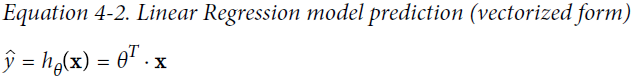
This can be written much more concisely using a vectorized form, as shown in Equation 4-2.

#################################################################################################
is one column if  is a horizontal (row) array/matrix
: is two dimension array likes/matrix
Note: sometimes, I like to use * , each row of represents an instance containing several features（columns）, the result of dot product( * ,) is a predicted labels vector, or each row is one element called a predicted label/class in the result （vertical, only one column with several rows, the actual labels are usually stored in last column of 2D dataset）.
#################################################################################################
 is one row if  is a vertical (column) array/matrix
: is two dimension array likes/matrix

But, here , xi is the ith feature value.  ( e.g.  X1 X2 X3  ... Xn),  thus i is the row index and the each row of x represents different features, each column of x represents eno instance. the result(horizontal) is only one row with several columns, the actual labels are usually stored in last row of 2D dataset

• θ is the model’s parameter vector, containing the bias term θ0 and the feature weights θ1 to θn.
•  is the transpose of θ (a row vector instead of a column vector).
• x is the instance’s feature vector, containing x0 to xn, with x0 always equal to 1.
• · x is the dot product of θT and x.
• hθ is the hypothesis function, using the model parameters θ.

Okay, that’s the Linear Regression model, so now how do we train it? Well, recall that training a model means setting its parameters so that the model best fits the training set. For this purpose, we first need a measure of how well (or poorly) the model fits the training data.  we saw that the most common performance measure of a regression model is the Root Mean Square Error (RMSE, 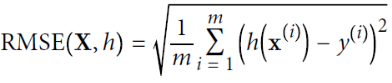, , is its label (the desired output value for that instance), the RMSE is more sensitive to outliers than level 1( the sum of absolutes MAE(Mean Absolute Error) since the higher the norm index of focuses on large values and neglects small ones) . Therefore, to train a Linear Regression model, you need to find the value of θ that minimizes the RMSE. In practice, it is simpler to minimize the Mean Square Error (MSE) than the RMSE, and it leads to the same result (because the value of θ that minimizes a function(MSE cost function) also minimizes its square root). 

####################################################
It is often the case that a learning algorithm will try to optimize a different function than the performance
measure used to evaluate the final model. This is generally because that function is easier to compute, because
it has useful differentiation properties差异化属性 that the performance measure lacks, or because we want to constrain约束the model during training, as we will see when we discuss regularization.

find the value of θ ==> minimizes MSE cost function ==> minimizes the RMSE

####################################################

The MSE of a Linear Regression hypothesis hθ on a training set X is calculated using Equation 4-3.
Equation 4-3. MSE cost function for a Linear Regression model 

Most of these notations were presented in (https://blog.csdn.net/Linli522362242/article/details/103387527). The only difference is that we write hθ instead of just h in order to make it clear that the model is parametrized by the vector θ. To simplify notations, we will just write MSE(θ) instead of MSE(X, hθ).

The Normal Equation正态方程

solve Normal Equation( has a closed-form solution) ==> find the value of θ ==> minimizes MSE cost function ==> minimizes the RMSE
or 
minimizes MSE cost function with gradient descent==> minimizes the RMSE

• The Linear Regression Model( weight w ==  ):
     

1. A regression equation of the form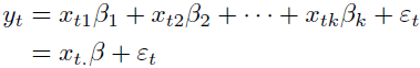（1, 2, 3, ..., k are features' indices)
   
   t = 1, 2, 3, ..., m are instances' indices and m is the total number of instances
   an unobservable random variable(error e== == )
   
   Note:   is just one instance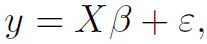
2. 
   wherein y = [y1, y2, ... , ym ] and e = [e1, e2,..., em],  are vectors of order m and =  is a matrix of order m * k. We shall assume that is a non-stochastic matrix with Rank(X) = k which requires that m > k.(k is the total number of features)

http://www.le.ac.uk/users/dsgp1/COURSES/MESOMET/ECMETXT/06mesmet.pdf

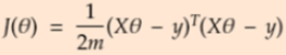
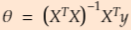
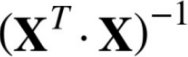
To find the value of θ that minimizes the cost function, there is a closed-form solution —in other words, a mathematical equation that gives the result directly. This is called the Normal Equation (Equation 4-4).

Equation 4-4. Normal Equation 
• is the value of θ that minimizes the cost function.
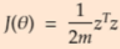
• y is the vector of target values containing y(1) to y(m).
############################################################
https://towardsdatascience.com/linear-regression-cost-function-gradient-descent-normal-equations-1d2a6c878e2c

Normal Equations

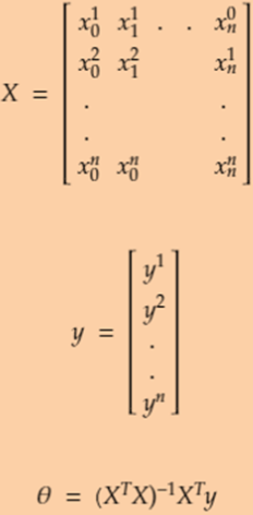
As Gradient Descent is an iterative process, Normal equations help to find the optimum solution in one go. They use matrix multiplication. The formula’s and notations are explained in the images. Below right image will explain what will be our X and y from our example. The first column of our X will always be 1 because it will be multiplied by Theta_0 or  which we know is our intercept to the axis's.    
X will be m*(k+1) matrix, m is the total number of instances, k is the total number of features.
Note: (error e== == ), each row of X is a instance, and y is the actual value, h(x) is the predicted value of y .

                                       

The derivation of the Normal Equation are explained in above right image. They use matrix notation and properties.

This image explains the

• ‘Theta’ matrix
• ‘x’ matrix
• hypothesis is expanded
• Using those matrix we can rewrite the hypothesis as given is last step

Figure 16(belowing left figure) explains the following

• We will replace our hypothesis in error function.  ( weight w ==  ==) 
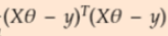
• We assume z matrix as given in step 2
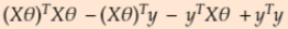
• Error Function can be rewritten as step 3. So if you multiply transpose of Z matrix with Z matrix. we will get our step 1 equation
• We can decompose z from step 2 as shown in step 4.
• By the property given in Step 6. We will rewrite z as given in Step 7. Capital X is also known as design matrix is transpose of small x
  The term  is just added for our convenience, which will make it easier to derive the gradient
  
• Substituting z in the equation==>
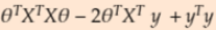
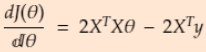
• Expand the error equation and then take derivative with respect to theta and equate it to 0. Minimum ==0 
• We will get out solution. As shown in below image
  ==>==>
  ==>
   
• ==
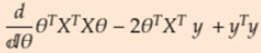
   #Find extreme values of partial derivatives 
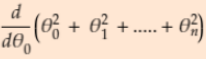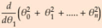•   = 2* , 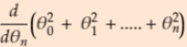=2*, ... =2*
• 1～n features(error e0== 0== ==w0 intercept with y-axis, see above)
• 
• Then=>==>x==>
   
• Minimum of  
• https://www.jianshu.com/p/36d808743087   Note: computational complexity:  == to   

############################################################
solve Normal Equation( has a closed-form solution) ==> find the value of θ ==> minimizes MSE cost function ==> minimizes the RMSE

Let’s generate some linear-looking data to test this equation on (Figure 4-1):

import numpy as np
# To plot pretty figures
%matplotlib inline
import matplotlib as mpl
import matplotlib.pyplot as plt

X = 2*np.random.rand(100,1) # 100rows 1column
 #4:intercept 3:weigtht # random error
y = 4 + 3*X + np.random.randn(100,1)

plt.plot(X, y, "b.") #blue dot
plt.xlabel("$X with 1 feature$", fontsize=18)
plt.ylabel("$y$", rotation=0, fontsize=18)
plt.axis([0,2, 0,15])
plt.title("Figure 4-1")
plt.show()

Now let’s compute using the Normal Equation. We will use the inv() function from NumPy’s Linear Algebra module (np.linalg) to compute the inverse of a matrix, and the dot() method for matrix multiplication:

X_b = np.c_[np.ones( (100,1) ), X] #add x0=1 to each instance, X0==1
X_b[:5]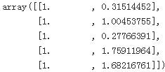 

#X = 2 * np.random.rand(100, 1)
#y = 4 + 3*X + np.random.randn(100,1) # np.random.randn(100,1) == Gaussian noise 
theta_best = np.linalg.inv( X_b.T.dot((X_b)) ).dot(X_b.T).dot(y)
theta_best

We would have hoped for θ0 = 4 and θ1 = 3 instead of θ0 = 4.11097362 and θ1 = 2.87496178. Close enough, but the noise made it impossible to recover the exact parameters of the original function.
Now you can make predictions using    

X_new = np.array([[0], [2]])
X_new_b = np.c_[np.ones((2,1)), X_new
               ]# add x0 =1 to each in each instance
X_new_b

 # X[:, 0]=[1 ,1]  

y_predict = X_new_b.dot(theta_best)
y_predict

plt.plot(X_new, y_predict, "r-", linewidth=2, label="Predictions")
plt.plot(X, y, "b.", label="Instances")
plt.xlabel("$x_1$", fontsize=18)
plt.ylabel("$y$", rotation=0, fontsize=18)
plt.axis([0,2, 0,15])
#plt.legend(["predictions","Instances",],loc="upper left", fontsize=14)
plt.legend(loc="upper left", fontsize=14)
plt.title("Figure 4-2. Linear Regression model predictions")
plt.show()

The equivalent code using Scikit-Learn looks like this:

from sklearn.linear_model import LinearRegression

lin_reg = LinearRegression()
lin_reg.fit(X,y)
lin_reg.intercept_, lin_reg.coef_  #theta_best

lin_reg.predict(X_new) #y_predict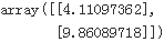

Computational Complexity ( the inverse of ==   )

The Normal Equation computes the inverse of , which is an n × n matrix (where n is the number of features). The computational complexity of inverting such a matrix is typically about  == to  (depending on the implementation). In other words, if you double the number of features, you multiply the computation time by roughly 5.3( = )  to
8() .

###############
WARNING
The Normal Equation gets very slow when the number of features grows large (e.g., 100,000).
###############
On the positive side, this equation is linear with regards to the number of instances in the training set (it is O(m)), so it handles large training sets efficiently, provided they can fit in memory.

Also, once you have trained your Linear Regression model (using the Normal Equation or any other algorithm), predictions are very fast: the computational complexity is linear with regards to 关于both the number of instances you want to make predictions on and the number of features. In other words, making predictions on twice as many instances (or twice as many features) will just take roughly twice as much time.

Now we will look at very different ways to train a Linear Regression model, better suited for cases where there are a large number of features, or too many training instances to fit in memory(Gradient Descent).

Gradient Descent

Gradient Descent is a very generic optimization algorithm capable of finding optimal solutions to a wide range of problems. The general idea of Gradient Descent is to tweak parameters iteratively in order to minimize a cost function.

Suppose you are lost in the mountains in a dense fog浓雾; you can only feel the slope of the ground below your feet. A good strategy to get to the bottom of the valley quickly is to go downhill in the direction of the steepest slope. This is exactly what Gradient Descent does: it measures the local gradient局部梯度 of the error function with regards to the parameter vector θ, and it goes in the direction of descending gradient. Once the gradient is zero, you have reached a minimum!

Concretely, you start by filling θ with random values (this is called random initialization), and then you improve it gradually, taking one baby step at a time, each step attempting to decrease the cost function (e.g., the MSE), until the algorithm converges to a minimum(see Figure 4-3).

An important parameter in Gradient Descent is the size of the steps, determined by the learning rate hyperparameter. If the learning rate is too small, then the algorithm will have to go through many iterations to converge, which will take a long time (see Figure 4-4).

On the other hand, if the learning rate is too high, you might jump across the valley and end up on the other side, possibly even higher up than you were before. This might make the algorithm diverge, with larger and larger values, failing to find a good solution (see Figure 4-5).

Finally, not all cost functions look like nice regular bowls. There may be holes洞, ridges山脊, plateaus 高原, and all sorts of irregular terrains地形, making convergence to the minimum very difficult. Figure 4-6 shows the two main challenges with Gradient Descent: if the random initialization starts the algorithm on the left, then it will converge to a local minimum, which is not as good as the global minimum. If it starts on the right, then it will take a very long time to cross the plateau, and if you stop too early you will never reach the global minimum.

Fortunately, the MSE cost function for a Linear Regression model happens to be a convex function, which means that if you pick any two points on the curve, the line segment joining them never crosses the curve该线段不会与曲线有第三个交点.This implies that there are no local minima, just one global minimum. It is also a continuous function with
a slope that never changes abruptly突然地. These two facts have a great consequence: Gradient Descent is
guaranteed to approach arbitrarily close the global minimum (if you wait long enough and if the learning rate is not too high).

In fact, the cost function has the shape of a bowl, but it can be an elongated被延长 bowl if the features have very different scales. Figure 4-7 shows Gradient Descent on a training set where features 1 and 2 have the same scale (on the left), and on a training set where feature 1 has much smaller values than feature 2 (on the right).Since feature 1 is smaller, it takes a larger change in θ1 to affect the cost function, which is why the bowl is elongated along the θ1 axis.

As you can see, on the left the Gradient Descent algorithm goes straight toward the minimum, thereby reaching it quickly, whereas on the right it first goes in a direction almost orthogonal to the direction of the global minimum, and it ends with a long
march down an almost flat valley. It will eventually reach the minimum, but it will take a long time.
#########################
WARNING
When using Gradient Descent, you should ensure that all features have a similar scale (e.g., using Scikit-Learn’s StandardScaler class), or else it will take much longer to converge.
#########################
This diagram also illustrates the fact that training a model means searching for a combination of model parameters that minimizes a cost function (over the training set). It is a search in the model’s parameter space: the more parameters a model has, the more dimensions this space has, and the harder the search is: searching for a needle in a 300-dimensional haystack干草堆 is much trickier than in three dimensions. Fortunately, since the cost function is convex in the case of Linear Regression, the needle is simply at the bottom of the bowl.
######################################################
https://towardsdatascience.com/linear-regression-cost-function-gradient-descent-normal-equations-1d2a6c878e2c

We will discuss the mathematical interpenetration of Gradient Descent but let’s understand some terms and notations as follows:

• alpha is learning rate which describes how big the step you take.
• Derivative gives you the slope of the line tangent to the ‘theta’ which can be either positive or negative and derivative tells us that we will increase or decrease the ‘theta’.
• Simultaneous update means that both theta should be updated simultaneously.

cost function : 
The term  which in the following equation that is just added for our convenience, which will make it easier to derive the gradient
       

Note: multiply the gradient vector by alpha  to determine the size of the downhill step : 
left theta is for next step (downhill step), right theta is currently theta value; Once the left theta == right theta, h(x) ==y means the gradient  equal to 0.
 
######################################################

Batch Gradient Descent

To implement Gradient Descent, you need to compute the gradient of the cost function with regards to each model parameter . In other words, you need to calculate how much the cost function will change if you change just a little bit. This is called a partial derivative. It is like asking “what is the slope of the mountain under my feet if I face east?” and then asking the same question facing north (and so on for all other dimensions, if you can imagine a universe with more than three dimensions). Equation 4-5 computes the partial derivative of the cost function with regards to parameter
, noted .
Note:cost function 
Equation 4-5. Partial derivatives of the cost function(start with  or i >=1)
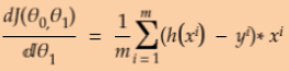== * 2 (without adding the term to the calculation process.)

Instead of computing these gradients individually, you can use Equation 4-6 to compute them all in one go. The gradient vector, noted , contains all the partial derivatives of the cost function (one for each model parameter, or weight wj).

Equation 4-1. Linear Regression model prediction (X0==1,  X0 * ==, the bias term also is w0 )
  

Equation 4-6. Gradient vector of the cost function ( for equation 4-5)
 Note: == *2

 (without adding the term to the calculation process.)
########################################
WARNING
Notice that this formula(Equation 4-6) involves calculations over the full training set X, at each Gradient Descent step! This is why the algorithm is called Batch Gradient Descent: it uses the whole batch of training data at every step. As a result it is terribly slow on very large training sets (but we will see much faster Gradient Descent algorithms shortly). However, Gradient Descent scales well with the number of features梯度下降的运算规模和特征的数量成正比; training a Linear Regression model when there are hundreds of thousands of features is much faster using Gradient Descent than using the Normal Equation.
########################################
Once you have the gradient vector, which points uphill, just go in the opposite direction to go downhill. This means subtracting from θ. This is where the learning rate η( η reads Eta, or )comes into play: multiply the gradient vector by η to determine the size of the downhill step (Equation 4-7).

Equation 4-7. Gradient Descent step 

Linear regression using batch gradient descent

eta = 0.1 # learning rate
n_iterations = 1000
m=100

theta = np.random.randn(2,1) # random initialization

for iteration in range(n_iterations):
    gradients = 2/m * X_b.T.dot( X_b.dot(theta) - y )
    theta = theta - eta*gradients
    
theta #lin_reg.intercept_, lin_reg.coef_  #theta_best

X_new_b.dot(theta) #predictions

Hey, that’s exactly what the Normal Equation found! Gradient Descent worked perfectly. But what if you had used a different learning rate eta? Figure 4-8 shows the first 10 steps of Gradient Descent using three different learning rates (the dashed line
represents the starting point).

theta_path_bgd = []
                         #weight,learning rate
def plot_gradient_descent(theta, eta, theta_path=None):
    m = len(X_b)
    plt.plot(X, y, "b.")
    
    n_iterations=1000
    for iteration in range(n_iterations):
        if iteration<10:
            y_predict=X_new_b.dot(theta)
            style = "b-" if iteration>0 else "r--" #r-- for start point
            plt.plot(X_new, y_predict, style)
        gradients = 2/m * X_b.T.dot( X_b.dot(theta)-y )
        theta = theta - eta*gradients
        if theta_path is not None:
            theta_path.append(theta)
    plt.xlabel("$x_1$", fontsize=18)
    plt.axis([0,2, 0,15])
    plt.title(r"$\eta = {}$".format(eta), fontsize=16)


np.random.seed(42)
theta = np.random.randn(2,1) # random initialization #weights

plt.figure( figsize=(10,4) )
plt.subplot(131); plot_gradient_descent(theta, eta=0.02)
plt.ylabel( "$y$", rotation=0, fontsize=18)
plt.subplot(132); plot_gradient_descent(theta, eta=0.1, theta_path=theta_path_bgd)
plt.subplot(133); plot_gradient_descent(theta, eta=0.5)

plt.show()

Figure 4-8. Gradient Descent with various learning rates

On the left, the learning rate is too low: the algorithm will eventually reach the solution( I believe: the algorithm can not find the final result if n_iterations=10), but it will take a long time(n_iterations>10).
In the middle, the learning rate looks pretty good: in just a few iterations, it has already converged to the solution.
On the right, the learning rate is too high: the algorithm diverges发散的, jumping all over the place and actually getting further and further away from the solution at every step.
##########################extra########################

theta_path_bgd = []
                         #weight,learning rate
def plot_gradient_descent(theta, eta, theta_path=None):
    m = len(X_b)
    plt.plot(X, y, "b.")
    
    n_iterations=1000
    for iteration in range(n_iterations):
        if iteration<200:########################
            y_predict=X_new_b.dot(theta)
            style = "b-" if iteration>0 else "r--" #r-- for start point
            plt.plot(X_new, y_predict, style)
        gradients = 2/m * X_b.T.dot( X_b.dot(theta)-y )
        theta = theta - eta*gradients
        if theta_path is not None:
            theta_path.append(theta)
    plt.xlabel("$x_1$", fontsize=18)
    plt.axis([0,2, 0,20])########################
    plt.title(r"$\eta = {}$".format(eta), fontsize=16)


np.random.seed(42)
theta = np.random.randn(2,1) # random initialization #weights

plt.figure( figsize=(10,4) )
plt.subplot(131); plot_gradient_descent(theta, eta=0.02)
plt.ylabel( "$y$", rotation=0, fontsize=18)
plt.subplot(132); plot_gradient_descent(theta, eta=0.1, theta_path=theta_path_bgd)
plt.subplot(133); plot_gradient_descent(theta, eta=0.5)

plt.show()

#######################################################
To find a good learning rate, you can use grid search (see https://blog.csdn.net/Linli522362242/article/details/103646927). However, you may want to limit the number of iterations so that grid search can eliminate models(kernel) that take too long to converge.
You may wonder how to set the number of iterations. If it is too low, you will still be far away from the optimal solution when the algorithm stops, but if it is too high, you will waste time while the model parameters do not change anymore. A simple solution is to set a very large number of iterations but to interrupt the algorithm when the gradient vector becomes tiny—that is, when its norm becomes smaller than a tiny number ϵ (called the tolerance,
 ==<ϵ )—because this happens when Gradient Descent has (almost) reached the minimum.
################################
Convergence Rate
When the cost function is convex and its slope does not change abruptly (as is the case for the MSE cost function), it can be shown that Batch Gradient Descent with a fixed learning rate has a convergence rate of . In other words, if you divide the tolerance ϵ by 10 (to have a more precise solution), then the algorithm will have to run about 10 times more iterations.
################################

Stochastic Gradient Descent

The main problem with Batch Gradient Descent is the fact that it uses the whole training set to compute the gradients at every step, which makes it very slow when the training set is large. At the opposite extreme, Stochastic Gradient Descent just picks a random instance in the training set at every step and computes the gradients based only on that single instance. Obviously this makes the algorithm much faster since it has very little data to manipulate at every iteration. It also makes it possible to train on huge training sets, since only one instance needs to be in memory at each iteration (SGD can be implemented as an out-of-core algorithm.)

On the other hand, due to its stochastic (i.e., random) nature, this algorithm is much less regular than Batch Gradient Descent: instead of gently decreasing平缓的下降 until it reaches the minimum, the cost function will bounce跳 up and down, decreasing only on average大体上. Over time it will end up very close to the minimum, but once it gets there it will continue to bounce around, never settling down (see Figure 4-9). So once the algorithm stops, the final parameter values are good, but not optimal.

         

When the cost function is very irregular (as in the right figure), this can actually help the algorithm jump out of local minima, so Stochastic Gradient Descent has a better chance of finding the global minimum than Batch Gradient Descent does.

Therefore randomness is good to escape from local optima, but bad because it means that the algorithm can never settle at the minimum. One solution to this dilemma 窘境is to gradually reduce the learning rate. The steps start out large (which helps make quick progress and escape local minima), then get smaller and smaller, allowing the algorithm to settle at the global minimum. This process is called simulated annealing模拟退火, because it resembles类似于 the process of annealing in metallurgy冶金 where molten熔融 metal is slowly cooled down. The function that determines the learning rate at each iteration
is called the learning schedule. If the learning rate is reduced too quickly, you may get stuck in a local minimum, or even end up frozen halfway to the minimum. If the learning rate is reduced too slowly, you may jump around the minimum for a long time and end up with a suboptimal solution if you halt training too early.

This code implements Stochastic Gradient Descent using a simple learning schedule:

theta_path_sgd = []
m=len(X_b)
np.random.seed(42)

n_epochs = 50
t0,t1= 5,50

def learning_schedule(t):
    return t0/(t+t1)

theta = np.random.randn(2,1)

for epoch in range(n_epochs): # n_epochs=50 replaces n_iterations=1000
    for i in range(m): # m = len(X_b)
        if epoch==0 and i<20:
            y_predict = X_new_b.dot(theta)
            style="b-" if i>0 else "r--"
            plt.plot(X_new,y_predict, style)######
            
        random_index = np.random.randint(m)  ##### Stochastic
        xi = X_b[random_index:random_index+1]
        yi = y[random_index:random_index+1]
        gradients = 2*xi.T.dot( xi.dot(theta) - yi ) ##### Gradient
        eta=learning_schedule(epoch*m + i) ############## e.g. 5/( (epoch*m+i)+50)
        theta = theta-eta * gradients  ###### Descent
        theta_path_sgd.append(theta)
        
        
plt.plot(X, y, "b.")
plt.xlabel("$x_1$", fontsize=18)
plt.ylabel("$y$", rotation=0, fontsize=18)
plt.title("Figure 4-10. Stochastic Gradient Descent first 10 steps")

plt.axis([0,2, 0,15])
plt.show()

By convention we iterate by rounds of m iterations(m = len(X_b)); each round is called an epoch.

While the Batch Gradient Descent code iterated 1,000 times through the whole training set, this code goes through the training set only 50 times and reaches a fairly good solution:

theta

theta_path_sgd[-10:]

Note that since instances are picked randomly, some instances may be picked several times per epoch while others may not be picked at all. If you want to be sure that the algorithm goes through every instance at each epoch, another approach is to shuffle the training set, then go through it instance by instance, then shuffle it again, and so
on. However, this generally converges more slowly.

To perform Linear Regression using SGD with Scikit-Learn, you can use the SGDRegressor class, which defaults to optimizing the squared error cost function. The following code runs 50 epochs, starting with a learning rate of 0.1 (eta0=0.1), using the default learning schedule (different from the preceding one), and it does not use any regularization (penalty=None; more details on this shortly):

from sklearn.linear_model import SGDRegressor
sgd_reg = SGDRegressor(tol=1e-3,max_iter=50, penalty=None, eta0=0.1, random_state=42)
sgd_reg.fit(X,y.ravel()) #y.ravel() converts y to one dimension with only one row

sgd_reg.intercept_, sgd_reg.coef_

Mini-batch Gradient Descent

The last Gradient Descent algorithm we will look at is called Mini-batch Gradient Descent. It is quite simple to understand once you know Batch and Stochastic Gradient Descent: at each step, instead of computing the gradients based on the full training set (as in Batch GD) or based on just one instance (as in Stochastic GD), Mini-batch GD computes the gradients on small random sets of instances called minibatches. The main advantage of Mini-batch GD over Stochastic GD is that you can get a performance boost from hardware optimization of matrix operations, especially when using GPUs.

theta_path_mgd = []

n_iterations = 50
minibatch_size=20

np.random.seed(42)
theta = np.random.randn(2,1) # Normal Distribution（0，1）=(u,sigma)

t0, t1 =200, 1000
def learning_schedule(t):
    return t0/(t+t1)

t=0
for epoch in range(n_iterations):
    shuffled_indices = np.random.permutation(m)
    X_b_shuffled = X_b[shuffled_indices]
    y_shuffled = y[shuffled_indices]
    for i in range(0,m, minibatch_size):
        t += 1
        xi = X_b_shuffled[i:i+minibatch_size]
        yi = y_shuffled[i:i+minibatch_size]
        gradients = 2/minibatch_size * xi.T.dot( xi.dot(theta)-yi)
        eta = learning_schedule(t)
        theta = theta-eta*gradients
        theta_path_mgd.append(theta)

theta

theta_path_bgd = np.array(theta_path_bgd)
theta_path_sgd = np.array(theta_path_sgd)
theta_path_mgd = np.array(theta_path_mgd)

plt.figure( figsize=(7,4) )
plt.plot(theta_path_sgd[:,0], theta_path_sgd[:,1], "y-s", linewidth=1, label="Stochastic")
plt.plot(theta_path_mgd[:,0], theta_path_mgd[:,1], "g-x", linewidth=1, label="Mini-batch" )
plt.plot(theta_path_bgd[:,0], theta_path_bgd[:,1], "b-o", linewidth=1, label="Batch")

plt.legend(loc="upper left", fontsize=16)
plt.xlabel(r"$\theta_0$", fontsize=20)
plt.ylabel(r"$\theta_1$", fontsize=20, rotation=0)
plt.axis([2.5, 4.5, 2.3, 3.9])
plt.title("Figure 4-11. Gradient Descent paths in parameter space")
plt.show()

The (Mini-batch Gradient Descent's) algorithm’s progress in parameter space is less erratic不规则的 than with SGD, especially with fairly large mini-batches. As a result, Mini-batch GD will end up walking around a bit closer to the minimum than SGD. But, on the other hand, it may be harder for it to escape from local minima (in the case of problems that suffer from local minima, unlike Linear Regression as we saw earlier). Figure 4-11 shows the paths taken by the three Gradient Descent algorithms in parameter space during training. They all end up near the minimum, but Batch GD’s path actually stops at the minimum, while both Stochastic GD and Mini-batch GD continue to walk around. However, don’t forget that Batch GD takes a lot of time to take each step, and Stochastic GD and Mini-batch GD would also reach the minimum if you used a good learning schedule.

#########################
While the Normal Equation can only perform Linear Regression, the Gradient Descent algorithms can be used to train many other models, as we will see.

#########################

Let’s compare the algorithms we’ve discussed so far for Linear Regression (recall that m is the number of training instances and n is the number of features); see Table 4-1.
Table 4-1. Comparison of algorithms for Linear Regression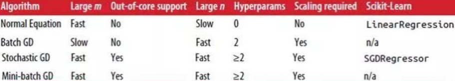

There is almost no difference after training: all these algorithms end up with very similar models and make predictions in exactly
the same way.

Polynomial Regression

What if your data is actually more complex than a simple straight line? Surprisingly, you can actually use a linear model to fit nonlinear data. A simple way to do this is to add powers of each feature as new features, then train a linear model on this extended set of features. This technique is called Polynomial Regression.

Let’s look at an example. First, let’s generate some nonlinear data, based on a simple quadratic equation9 (plus some noise; see Figure 4-12): 

import numpy as np
import numpy.random as rnd

np.random.seed(42)

m=100
X = 6*np.random.rand(m,1) -3 #np.random.rand() is a uniform distribution over [0.0, 1) #[-3,3)
                       #noise
y = 0.5*X**2 + X + 2 + np.random.randn(m,1)

plt.plot(X,y, "b.")
plt.xlabel("$x_1$", fontsize=18)
plt.ylabel("$y$", rotation=0, fontsize=18)
plt.axis([-3,3, 0,10])
plt.title("Figure 4-12. Generated nonlinear and noisy dataset")
plt.show()

Clearly, a straight line will never fit this data properly. So let’s use Scikit-Learn’s PolynomialFeatures class to transform our training data, adding the square (2nd-degree polynomial) of each feature in the training set as new features (in this case there is just one feature):

from sklearn.preprocessing import PolynomialFeatures
poly_features = PolynomialFeatures(degree=2, include_bias=False) #2 Dimensions data, so set degree=2
X_poly = poly_features.fit_transform(X)
X[:3]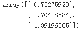

X_poly[:3] #-0.75275929 * -0.75275929==0.56664654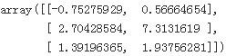

X_poly now contains the original feature of X plus the square of this feature. Now you can fit a LinearRegression model to this extended training data (Figure 4-13):

lin_reg = LinearRegression()
lin_reg.fit(X_poly,y)
lin_reg.intercept_, lin_reg.coef_

X_new = np.linspace(-3,3,100).reshape(100,1)
X_new_poly = poly_features.transform(X_new)
y_new = lin_reg.predict(X_new_poly)

plt.plot(X,y,"b.")

plt.plot(X_new, y_new, "r-", linewidth=2, label="Predictions")
plt.xlabel("$x_1$", fontsize=18)
plt.ylabel("$y$", rotation=0, fontsize=18)
plt.legend(loc="upper left", fontsize=14)
plt.axis([-3,3,0,10])
plt.title("Figure 4-13. Polynomial Regression model predictions")
plt.show()

Not bad: the model estimates when in fact the original function was .

Note that when there are multiple features, Polynomial Regression is capable of finding relationships between features (which is something a plain Linear Regression model cannot do). This is made possible by the fact that PolynomialFeatures also adds all combinations of features up to the given degree阶数. For example, if there were two features a and b, PolynomialFeatures with degree=3(3 阶) would not only add the features , and , but also the combinations , and .
#########################
WARNING
PolynomialFeatures(degree=d) transforms an array containing features into an array containing features, where n!
is the factorial of n, equal to 1 × 2 × 3 × ... × n. Beware of the combinatorial explosion of the number of features!
#########################

Learning Curves

https://blog.csdn.net/Linli522362242/article/details/104070847