用keras理解循环神经网络

概述

本博客用伪代码来代替繁杂的数学公式，让跟多人能够避开令人眼花的复杂公式，通过伪代码快速理解RNN和LSTM RNN的计算步骤。然后用通俗的话来解释其工作原理，达到对其原理和结构的理解。然后用RNN和LSTM RNN做一个简单的应用，并分析其差异和优劣。

理解RNN

具体的RNN背景和数学推导，大家可以参考这篇博客
首先在结构上来感受一下RNN，如下图所示

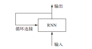
我们用伪代码来解释其结构

#网络初始状态
state_t = 0   
for input_t in input_sequence:    
    output_t = activation(dot(W, input_t) + dot(U, state_t) + b)
    state_t = output_t

其中我们输入的样本形状为(timesteps, input_features)，而整个网络对时间步（timestep）进行遍历，在每个时间步，它考虑t 时刻的当前状态与t时刻的输入［形状为(input_ features,)］，对二者计算得到t 时刻的输出。然后，我们将下一个时间步的状态设置为上一个时间步的输出。

为了进一步了解其计算，我们用numpy来实现RNN的向前传播：

import numpy as np
timesteps = 100
input_features = 32
output_features = 64
inputs = np.random.random((timesteps, input_features))
state_t = np.zeros((output_features,))
W = np.random.random((output_features, input_features))
U = np.random.random((output_features, output_features))
b = np.random.random((output_features,))
successive_outputs = []
for input_t in inputs:
	output_t = np.tanh(np.dot(W, input_t) + np.dot(U, state_t) + b)
	successive_outputs.append(output_t)
	state_t = output_t
final_output_sequence = np.stack(successive_outputs, axis=0)

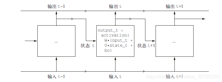
按时间展开，得到下图

理解LSTM

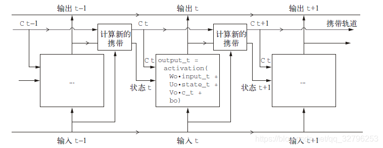
LSTM 层是SimpleRNN 层的一种变体，它增加了一种携带信息跨越多个时间步的方法。假设有一条传送带，其运行方向平行于你所处理的序列。序列中的信息可以在任意位置跳上传送带，然后被传送到更晚的时间步，并在需要时原封不动地跳回来。这实际上就是LSTM 的原理：它保存信息以便后面使用，从而防止较早期的信号在处理过程中逐渐消失。

而LSTM是在RNN的基础上添加了一个额外的数据流

然后对在对 $c_t$进行计算和处理，作为输入函数的一部分，伪代码如下

output_t = activation(dot(state_t, Uo) + dot(input_t, Wo) + dot(C_t, Vo) + bo)
#输入门
i_t = activation(dot(state_t, Ui) + dot(input_t, Wi) + bi)
遗忘门
f_t = activation(dot(state_t, Uf) + dot(input_t, Wf) + bf)
#候选记忆单元
k_t = activation(dot(state_t, Uk) + dot(input_t, Wk) + bk)

c_t+1 = i_t * k_t + c_t * f_t

时间展开图如下：

如果我们非要解释每一个计算目的，我认为是没有必要的。因为这些运算的实际效果是由参数化权重决定的，而权重是以端到端的方式进行学习，每次训练都要从头开始，不可能为某个运算赋予特定的目的。RNN 单元的类型（如前所述）决定了你的假设空间，即在训练期间搜索良好模型配置的空间，但它不能决定RNN 单元的作用，那是由单元权重来决定的。同一个单元具有不同的权重，可以实现完全不同的作用。因此，组成RNN 单元的运算组合，最好被解释为对搜索的一组约束，而不是一种工程意义上的设计。

对于研究人员来说，这种约束的选择（即如何实现RNN 单元）似乎最好是留给最优化算法来完成（比如遗传算法或强化学习过程），而不是让人类工程师来完成。在未来，那将是我们构建网络的方式。总之，你不需要理解关于LSTM 单元具体架构的任何内容。作为人类，理解它不应该是你要做的。你只需要记住LSTM 单元的作用：允许过去的信息稍后重新进入，从而解决梯度消失问题。

用keras实现RNN和LSTM例子

首先我们选择keras内置的IMDB数据集进行情感分类，关于这个数据集及相关实验可以参考上一篇博客,如果因为网络问题下载失败，请移步这里。

首先准备IMDB数据集

from keras.datasets import imdb
from keras.preprocessing import sequence

max_features = 10000  # number of words to consider as features
maxlen = 500  # cut texts after this number of words (among top max_features most common words)
batch_size = 32

print('Loading data...')
(input_train, y_train), (input_test, y_test) = imdb.load_data(num_words=max_features)
print(len(input_train), 'train sequences')
print(len(input_test), 'test sequences')

print('Pad sequences (samples x time)')
input_train = sequence.pad_sequences(input_train, maxlen=maxlen)
input_test = sequence.pad_sequences(input_test, maxlen=maxlen)
print('input_train shape:', input_train.shape)
print('input_test shape:', input_test.shape)

构建网络并训练

from keras.layers import Dense

model = Sequential()
model.add(Embedding(max_features, 32))
model.add(SimpleRNN(32))
model.add(Dense(1, activation='sigmoid'))

model.compile(optimizer='rmsprop', loss='binary_crossentropy', metrics=['acc'])
history = model.fit(input_train, y_train,
                    epochs=10,
                    batch_size=128,
                    validation_split=0.2)

可视化

import matplotlib.pyplot as plt

acc = history.history['acc']
val_acc = history.history['val_acc']
loss = history.history['loss']
val_loss = history.history['val_loss']

epochs = range(len(acc))

plt.plot(epochs, acc, 'bo', label='Training acc')
plt.plot(epochs, val_acc, 'b', label='Validation acc')
plt.title('Training and validation accuracy')
plt.legend()

plt.figure()

plt.plot(epochs, loss, 'bo', label='Training loss')
plt.plot(epochs, val_loss, 'b', label='Validation loss')
plt.title('Training and validation loss')
plt.legend()

plt.show()

改为LSTM模型

from keras.layers import LSTM

model = Sequential()
model.add(Embedding(max_features, 32))
model.add(LSTM(32))
model.add(Dense(1, activation='sigmoid'))

model.compile(optimizer='rmsprop',
              loss='binary_crossentropy',
              metrics=['acc'])
history = model.fit(input_train, y_train,
                    epochs=10,
                    batch_size=128,
                    validation_split=0.2)

可以发现RNN准确率为0.85而LSTM 的准确率为0.9，LSTM要优于RNN。