PyTorch入门（二）卷积神经网络的案例分析 AlexNet、VGGNet、GoogLeNet、ResNet

PyTorch入门

LeNet-5
AlexNet
VGG-16
GoogleNet
ResNet
其他
参考链接

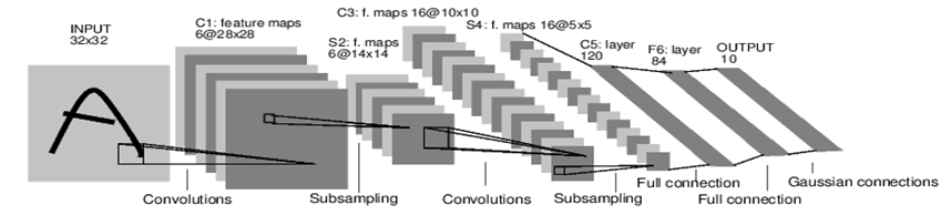
LeNet-5

LeNet-5 可以进行MNIST手写数字识别

网络基本结构
input (1) $\longrightarrow$ conv1 (6) $\longrightarrow$ pool1 (6) $\longrightarrow$ conv2 (16) $\longrightarrow$ pool2 (16) $\longrightarrow$ fc3 $\longrightarrow$ fc4 $\longrightarrow$ fc5 $\longrightarrow$ softmax
括号内的数字代表该层的通道数
特点
1. 卷积层-池化层被认为能够提取输入图像的平移不变特征
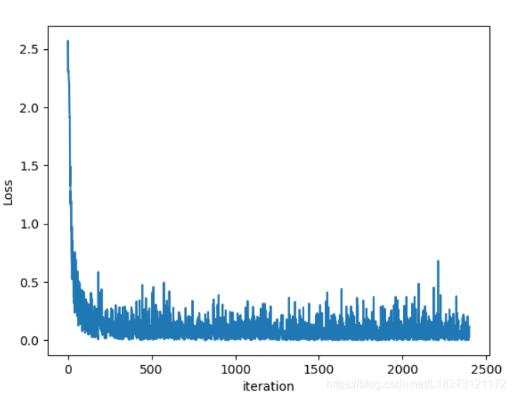
损失函数的曲线图如下：

上代码

#CNN进行MNIST手写数字集的识别
import torch
import torch.nn as nn
import torch.nn.functional as F
import torch.utils.data as data
import torchvision
import torchvision.transforms as transforms
import matplotlib.pyplot as plt

#Hyper parameters
LR = 0.01
EPOCH = 2
BATCH_SIZE = 50
DOWNLOAD_MNIST = False
transforms = transforms.ToTensor()
#准备训练集和测试集
train_set = torchvision.datasets.MNIST(
    root='./data/MNIST',
    train=True,
    transform=transforms,
    download=DOWNLOAD_MNIST
)
train_loader = data.DataLoader(
    dataset=train_set,
    batch_size=BATCH_SIZE,
    shuffle=True
)
#测试集只取2000个数据
test_set = torchvision.datasets.MNIST(
    root = './data/MNIST',
    train=False,
    transform=transforms,
    download=DOWNLOAD_MNIST)

test_loader = data.DataLoader(
    dataset=test_set,
    batch_size= 2000,
    shuffle=True
)
test_loader = iter(test_loader).next()

#搭建网络
class Net(nn.Module):
    def __init__(self):
        super(Net,self).__init__()
        self.conv1 = nn.Sequential(         #input shape: (1,28,28)    (C,H,W)
            nn.Conv2d(1,16,5,1,2),          # ->(16,28,28)
            nn.ReLU(),
            nn.MaxPool2d(2,2)               # ->(16,14,14)
        )
        self.conv2 = nn.Sequential(
            nn.Conv2d(16,32,5,1,2),         # ->(32,14,14)
            nn.ReLU(),
            nn.MaxPool2d(2,2)               # ->(32,7,7)
        )
        # self.fc1 = nn.Linear(32*7*7,400)    # ->(1,400)
        # self.fc2 = nn.Linear(400,120)       # ->(1,120)
        # self.fc3 = nn.Linear(120,10)        # ->(1,10)
        self.fc = nn.Linear(32*7*7,10)

    def forward(self,x):
        # x = self.conv1(x)
        # x = self.conv2(x)
        # x = x.view(-1,32*7*7)
        # x = F.relu(self.fc1(x))
        # x = F.relu(self.fc2(x))
        # x = self.fc3(x)
        # return x
        x = self.conv1(x)
        x = self.conv2(x)
        x = x.view(-1,32*7*7)
        x = self.fc(x)
        return x

net = Net()

#定义损失函数和优化器

criterion = nn.CrossEntropyLoss()
optimizer = torch.optim.Adam(net.parameters(),lr=LR,betas=(0.9,0.99))

#训练网络
loss_his = []
for epoch in range(EPOCH):
    for i,(inputs,labels) in enumerate(train_loader):
        #inputs: 图像 Tensor(50,1,28,28)
        #labels: 标签 Tensor(50)

        optimizer.zero_grad()
        outputs = net(inputs)     #Tensor(50,10)
        #loss是一个批次内所有样本loss的平均值
        #loss是一个值（1维的Tensor）
        loss = criterion(outputs,labels)
        loss.backward()
        optimizer.step()
        loss_his.append(loss)

        if (i % 50) == 0:
           #每50批次计算一次loss和accuracy并输出
            inputs,labels = test_loader
            outputs = net(inputs)
            _, predicted = torch.max(outputs,1)
            accuracy = (predicted == labels).sum().item()/labels.size(0)*100
            print('Epoch: ',epoch,'|loss: %.3f'%(loss.data.numpy()),'|Accuracy: %.2f%%'%(accuracy))

print('Training Finished !')

#显示预测示例
images,labels = test_loader
images = images[:10]
labels = labels[:10]
outputs = net(images)
_,predicted = torch.max(outputs,1)
print('GroundTruth:\n',labels.numpy())
print('Predicted Types:\n',predicted.numpy())

plt.plot(loss_his)
plt.xlabel('iteration')
plt.ylabel('Loss')
plt.show()

输出结果：

Epoch:  0 |loss: 2.310 |Accuracy: 9.55%
Epoch:  0 |loss: 0.372 |Accuracy: 87.20%
Epoch:  0 |loss: 0.260 |Accuracy: 94.40%
Epoch:  0 |loss: 0.037 |Accuracy: 95.90%
Epoch:  0 |loss: 0.077 |Accuracy: 96.75%
Epoch:  0 |loss: 0.072 |Accuracy: 95.80%
Epoch:  0 |loss: 0.049 |Accuracy: 96.75%
Epoch:  0 |loss: 0.087 |Accuracy: 96.25%
Epoch:  0 |loss: 0.104 |Accuracy: 97.10%
Epoch:  0 |loss: 0.197 |Accuracy: 96.65%
Epoch:  0 |loss: 0.033 |Accuracy: 97.20%
Epoch:  0 |loss: 0.196 |Accuracy: 97.10%
Epoch:  0 |loss: 0.015 |Accuracy: 96.95%
Epoch:  0 |loss: 0.047 |Accuracy: 96.95%
Epoch:  0 |loss: 0.119 |Accuracy: 97.30%
Epoch:  0 |loss: 0.075 |Accuracy: 96.60%
Epoch:  0 |loss: 0.081 |Accuracy: 97.35%
Epoch:  0 |loss: 0.048 |Accuracy: 96.50%
Epoch:  0 |loss: 0.025 |Accuracy: 97.20%
Epoch:  0 |loss: 0.024 |Accuracy: 96.65%
Epoch:  0 |loss: 0.004 |Accuracy: 97.30%
Epoch:  0 |loss: 0.023 |Accuracy: 97.25%
Epoch:  0 |loss: 0.004 |Accuracy: 97.50%
Epoch:  0 |loss: 0.170 |Accuracy: 97.90%
Epoch:  1 |loss: 0.024 |Accuracy: 96.95%
Epoch:  1 |loss: 0.181 |Accuracy: 96.95%
Epoch:  1 |loss: 0.036 |Accuracy: 97.65%
Epoch:  1 |loss: 0.082 |Accuracy: 97.75%
Epoch:  1 |loss: 0.026 |Accuracy: 97.30%
Epoch:  1 |loss: 0.127 |Accuracy: 97.75%
Epoch:  1 |loss: 0.220 |Accuracy: 96.80%
Epoch:  1 |loss: 0.412 |Accuracy: 97.55%
Epoch:  1 |loss: 0.166 |Accuracy: 97.70%
Epoch:  1 |loss: 0.022 |Accuracy: 97.40%
Epoch:  1 |loss: 0.047 |Accuracy: 97.75%
Epoch:  1 |loss: 0.002 |Accuracy: 97.55%
Epoch:  1 |loss: 0.023 |Accuracy: 97.45%
Epoch:  1 |loss: 0.046 |Accuracy: 97.80%
Epoch:  1 |loss: 0.084 |Accuracy: 97.35%
Epoch:  1 |loss: 0.090 |Accuracy: 97.75%
Epoch:  1 |loss: 0.005 |Accuracy: 97.85%
Epoch:  1 |loss: 0.188 |Accuracy: 97.40%
Epoch:  1 |loss: 0.068 |Accuracy: 97.80%
Epoch:  1 |loss: 0.023 |Accuracy: 97.40%
Epoch:  1 |loss: 0.114 |Accuracy: 97.45%
Epoch:  1 |loss: 0.040 |Accuracy: 97.80%
Epoch:  1 |loss: 0.072 |Accuracy: 97.40%
Epoch:  1 |loss: 0.004 |Accuracy: 98.05%
Training Finished !
GroundTruth:
 [0 4 1 0 5 9 3 8 5 6]
Predicted Types:
 [0 4 1 0 5 9 3 8 5 6]

AlexNet

网络基本结构：

input (3,224,224) $\longrightarrow$ conv1 (96,55,55) $\longrightarrow$ pool1 (96,27,27) $\longrightarrow$ conv2 (256,27,27) $\longrightarrow$ pool2 (256,13,13) $\longrightarrow$ conv3 (384,13,13) $\longrightarrow$ conv4 (384,13,13) $\longrightarrow$ conv5(256,13,13) $\longrightarrow$ pool (256,6,6) $\longrightarrow$ dropout $\longrightarrow$ fc6 (4096) $\longrightarrow$ dropout $\longrightarrow$ fc7 (4096) $\longrightarrow$ fc8 (1000) $\longrightarrow$ softmax

括号中表示每层激活值的shape，即（C, H, W）
特点
(1) 使用ReLU激活函数，解决梯度消失的问题
(2) 使用Dropout层来进行正则化，防止网络的过拟合
(3) 采用两个GPU进行并行运算
(4) 采用Local Response Normalization (LRN) 局部响应归一化层

上代码

#AlexNet网络结构

import torch
import torchvision
import torch.nn as nn
import torchvision.transforms as tranforms
import numpy as np


#搭建网络
class Net(nn.Module):
    def __init__(self,num_classes):
        super(Net,self).__init__()
        self.conv1 = nn.Sequential(     # -> (224,224,3)
            nn.Conv2d(3,96,11,4),       # -> (55,55,96)
            nn.ReLU(),
            nn.MaxPool2d(3,2)           # -> (27,27,96)
        )
        self.conv2 = nn.Sequential(
            nn.Conv2d(96,256,5,1,2),    # -> (27,27,256)
            nn.ReLU(),
            nn.MaxPool2d(3,2)           # -> (13,13,256)
        )
        self.conv3 = nn.Sequential(
            nn.Conv2d(256,384,3,1,1),   # -> (13,13,384)
            nn.ReLU()
        )
        self.conv4 = nn.Sequential(
            nn.Conv2d(384,384,3,1,1),   # -> (13,13,384)
            nn.ReLU()
        )
        self.conv5 = nn.Sequential(
            nn.Conv2d(384,256,3,1,1),    # -> (13,13,256)
            nn.ReLU(),
            nn.MaxPool2d(3,2),           # -> (6,6,256)
            nn.Dropout()
        )
        self.fc6 = nn.Sequential(
            nn.Linear(256*6*6,4096),    # -> (4096)
            nn.ReLU(),
            nn.Dropout()
        )
        self.fc7 = nn.Sequential(
            nn.Linear(4096,4096),       # -> (4096)
            nn.ReLU()
        )
        self.fc8 = nn.Linear(4096,num_classes)

    def forward(self,x):
        x = self.conv1(x)
        x = self.conv2(x)
        x = self.conv3(x)
        x = self.conv4(x)
        x = self.conv5#ssss(x)
        x = x.view(x.size(0),6*6*256)
        x = self.fc6(x)
        x = self.fc7(x)
        x = self.fc8(x)
        return x

net = Net(1000)
print(net)

VGG-16

网络基本结构

2.特点
（1）卷积核采用小卷积核：3 x 3 卷积 2 x 2 池化
（2）卷积层都是same convolution，不改变图片的高和宽，只将通道数进行成倍增加
（3）池化层的参数设置： f = 2 ，s = 2，p = 0，所以图片经过池化后高和宽都减半
（4）参数量大：138milion 个参数，大部分集中在全连接层

GoogleNet

GoogleNet又叫InceptionNet，网络主要由Inception 模块组成
Inception 模块： 由若干个不同尺寸的过滤器组成，运用这些过滤器对输入进行卷积和池化，然后将输出结果按照深度拼接在一起形成输出层

网络基本结构
如下图
特点
（1）采用多个过滤器： 有1x1、3x3、5x5三种尺寸的卷积和3x3的池化，不需要人为的去设计过滤器的尺寸，相当于让网络自己去学习过滤器的种类和尺寸
（2）采用1x1卷积： 1x1卷积在不改变图片高和宽的前提下，可以压缩通道的数目，从而达到减少参数的数量和计算过程中的乘法次数

上代码

#GoogleNet网络结构
# GoogleNet也叫InceptionNet，整个网络有多个Inception 模块组成

#这里只搭建Inception模块
import torch
import torch.nn as nn

class InceptionNet(nn.Module):
    def __init__(self,in_channels):
        super(InceptionNet,self).__init__()
        self.branch1x1 = nn.Sequential(
            nn.Conv2d(in_channels,64,1),
            nn.BatchNorm2d(64,eps = 0.001),
            nn.ReLU()
        )
        self.branch3x3 = nn.Sequential(
            nn.Conv2d(in_channels,96,1),
            nn.BatchNorm2d(96, eps = 0.001),
            nn.ReLU(),
            nn.Conv2d(96, 128, 3, 1, 1),
            nn.BatchNorm2d(128, eps=0.001),
            nn.ReLU()
        )
        self.branch5x5 = nn.Sequential(
            nn.Conv2d(in_channels,16,1),
            nn.BatchNorm2d(16, eps = 0.001),
            nn.ReLU(),
            nn.Conv2d(16,32,5,1,2),
            nn.BatchNorm2d(32, eps=0.001),
            nn.ReLU()
        )
        self.branch_pool = nn.Sequential(
            nn.MaxPool2d(3,1,1),
            nn.BatchNorm2d(in_channels, eps=0.001),
            nn.ReLU(),
            nn.Conv2d(in_channels,32,1),
            nn.BatchNorm2d(32, eps=0.001),
            nn.ReLU()
        )

        def forward(self,x):
            branch_1x1 = self.branch1x1(x)
            branch_3x3 = self.branch3x3(x)
            branch_5x5 = self.branch5x5(x)
            branch_pool= self.branch_pool(x)
            branch = [branch_1x1,branch_3x3,branch_5x5,branch_pool]
            x = torch.cat(branch,1)
            return x


net = InceptionNet(3)
print(net)

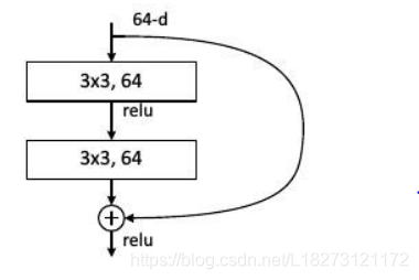
ResNet

ResNet 提出残差模块（Residual Block）, 解决网络加深后训练难度增大的现象，有效缓解反向传播时由于深度过深导致的梯度消失现象，这使得网络加深之后性能不会变差。

基本结构
特点
（1）Residual Block： 随着深度的增加，模型在训练集上的正确率不会下降，而误差会一直减小，从而使得可以训练更深层的神经网络
（2）大量使用批处理化： Batch Normalization
准确率
使用ResNet去进行CIFAR10数据集的图片分类

训练集上的accuracy：90.00 %
测试集上的accuracy：78.68 %

上代码

ResNet.py

#ResNet网络

#接口：ResNet(layers, num_classes)
# layers: 每个残差层中残差模块的数目
# num_classes:分类的类别数

import torch
import torch.nn as nn
import torch.nn.functional as F

#先搭建残差模块
class ResModule(nn.Module):
    def __init__(self,in_channels,out_channels,stride = 1):
        super(ResModule,self).__init__()
        self.conv1 = nn.Sequential(
            nn.Conv2d(in_channels,out_channels,3,stride,1),
            nn.BatchNorm2d(out_channels, eps = 0.001),
            nn.ReLU()
        )
        self.conv2 = nn.Sequential(
            nn.Conv2d(out_channels,out_channels,3,1,1),
            nn.BatchNorm2d(out_channels, eps = 0.001)

        )
        #对residual进行卷积，保证residual和x 在各个维度上的值相等
        self.downsample = nn.Sequential(
            nn.Conv2d(in_channels, out_channels, 3, stride, 1),
            nn.BatchNorm2d(out_channels, eps=0.001)
        )

    def forward(self,x):
        residual = x
        x = self.conv1(x)
        x = self.conv2(x)
        if  (x.size(1) != residual.size(1)) or (x.size(2) != residual.size(2)):
            # x的在各个维度上的值发生变化时
            residual = self.downsample(residual)
        x = F.relu(x+residual)
        return  x

#再搭建残差网络
class ResNet(nn.Module):
    def __init__(self,layers,num_classes):
        #block: 残差模块类
        # layers: 每个残差层中残差模块的数目
        # num_classes:分类的类别数
        super(ResNet,self).__init__()
        self.in_channels = 16
        self.conv = nn.Sequential(                                  # -> (3,32,32)
            nn.Conv2d(3,self.in_channels,3,1,1),                    # -> (16,32,32)
            nn.BatchNorm2d(self.in_channels, eps = 0.001),
            nn.ReLU()
        )
        self.resLayer1 = self.make_layer(ResModule,layers[0],32,1)        # -> (32,32,32)
        self.resLayer2 = self.make_layer(ResModule, layers[1], 64,2)      # -> (64,16,16)
        self.resLayer3 = self.make_layer(ResModule, layers[2], 128,2)     # -> (128,8,8)
        self.maxPool = nn.MaxPool2d(2,2)                              # -> (128,4,4)
        self.fc1 = nn.Linear(128*4*4,500)                             # -> (500)
        self.fc2 = nn.Linear(500,120)                                 # -> (120)
        self.fc3 = nn.Linear(120,num_classes)                         # -> (num_classes)


    def make_layer(self,block,num_modules,out_channels,stride = 1):
        #block: 残差模块类
        #num_modules: 需要搭建的残差模块的数目

        resLayer = []
        resLayer.append(
            block(self.in_channels,out_channels,stride)
        )
        for i in range(num_modules):
            resLayer.append(
                block(out_channels,out_channels)
            )
        self.in_channels = out_channels

        return nn.Sequential(
            *resLayer
        )

    def forward(self,x):
        x = self.conv(x)
        x = self.resLayer1(x)
        x = self.resLayer2(x)
        x = self.resLayer3(x)
        x = self.maxPool(x)
        x = x.view(x.size(0),-1)
        x = self.fc1(x)
        x = self.fc2(x)
        x = self.fc3(x)
        return x

classification_CIFAR10.py

#使用残差结构来图像分类
#数据集：CIFAR10
import ResNet
import torch
import torch.nn as nn
import torch.functional as F
import torchvision
import torchvision.transforms as transforms
import torch.utils.data as data
import numpy as np
import matplotlib.pyplot as plt

#超参数
EPOCH = 20
LR = 0.01
BATCH_SIZE = 60
DOWNLOAD = False

#准备数据集CIFAR10
def get_data():
    #数据转换器
    train_transform = transforms.Compose(
        [transforms.ToTensor(),
         transforms.Normalize([0.5,0.5,0.5],[0.5,0.5,0.5])
         # transforms.Scale(4),
         # transforms.RandomHorizontalFlip(),
         # transforms.RandomCrop(32)
        ]
    )
    test_transform = transforms.Compose(
        [transforms.ToTensor(),
         transforms.Normalize([0.5,0.5,0.5],[0.5,0.5,0.5])]
    )

    train_set = torchvision.datasets.CIFAR10(
        root='./data/CIFAR10',
        train = True,
        download=DOWNLOAD,
        transform = train_transform
    )
    train_loader = data.DataLoader(
        dataset=train_set,
        batch_size=BATCH_SIZE,
        shuffle=True
    )
    test_set = torchvision.datasets.CIFAR10(
        root='./data/CIFAR10',
        train = False,
        download=DOWNLOAD,
        transform = test_transform
    )
    test_loader = data.DataLoader(
        dataset=test_set,
        batch_size=BATCH_SIZE,
        shuffle=True
    )
    return train_loader,test_loader

#搭建网络
net = ResNet.ResNet([3,4,5],10)
net = net.cuda()
#定义优化器和损失函数
criterion = nn.CrossEntropyLoss()
criterion = criterion.cuda()
optimizer = torch.optim.Adam(net.parameters(), lr = LR, betas=(0.9,0.99))

train_loader,test_loader = get_data()
# #训练网络
# print('开始训练网络...\n')
# print('网络是否在cuda上训练:\n')
# print(next(net.parameters()).is_cuda)
# losses_his = []
# for epoch in range(EPOCH):
#     for i, (images,labels) in enumerate(train_loader):
#         images = images.cuda()
#         labels = labels.cuda()
#         optimizer.zero_grad()
#         outputs = net(images)
#         loss = criterion(outputs,labels)
#         loss.backward()
#         optimizer.step()
#
#         losses_his.append(loss.item())
#
#         if (i+1) % 50 == 0:
#             #每隔50批次输出一次loss和accuracy
#             _, predicted = torch.max(outputs,1)
#             correct = (predicted == labels).sum().item()
#             trian_accuracy = correct/labels.size(0)*100
#
#             print('Epoch: %d | Batch: [%d,%d] | Loss: %.4f | Accuracy: %.2f %% '%(epoch,i+1,1000,loss.data.item(),trian_accuracy) )

# torch.save(net.state_dict(),'./models/ResNet_CIFAR10.pkl')
net.load_state_dict(torch.load('./models/ResNet_CIFAR10.pkl'))

#测试网络
num_correct = 0
total_test = 0
net.eval()
print('开始测试网络...')
with torch.no_grad():
    for (images,labels) in test_loader:
        images = images.cuda()
        labels = labels.cuda()
        outputs = net(images)
        _, predicted = torch.max(outputs,1)
        num_correct += (predicted == labels).sum().item()
        total_test += labels.size(0)
    test_accuracy = num_correct/ total_test*100
print('Test set: Accuracy: %.2f %%'%(test_accuracy))

#输出部分测试用例
classes = ('plane','car','bird','cat','deer','dog','frog','horse','ship','truch')
num_show = 10       #展示的测试用例个数
#test_loader是个可迭代数据对象，每个元素包含两个张量。
# 一个是图像张量，其维度为：（60,3,32,32）;一个是标签张量，其维度是：（60）
data = iter(test_loader).next()
images,labels = data                #images是图片张量，维度：(60,3,32,32)  labels是标签张量，维度：(60)
images = images[:num_show]
labels = labels[:num_show]
images = images.cuda()
labels = labels.cuda()
outputs = net(images)
_, predicted = torch.max(outputs,1)
print('Ground Truth:')
print(' '.join('%5s'% classes[labels[i]] for i in range(num_show)))
print('Predicted Types:')
print(' '.join('%5s'% classes[predicted[i]] for i in range(num_show)))

#可视化
plt.plot(losses_his)
plt.title('Loss Function Curve')
plt.xlabel('iteration')
plt.ylabel('Loss')
plt.show()

输出

Test set: Accuracy: 78.68 %
Ground Truth:
  cat plane   dog plane   car  deer   dog truch   car   dog
Predicted Types:
  cat plane   dog plane   car  deer   dog truch   car   cat

其他

#使用CNN进行图像分类
#数据集：CIFAR-10
import torch
import  torch.nn as nn      #构建网络的常用包
import torchvision          #包含常用数据集包
import torchvision.transforms as transforms   #数据格式转化包


#加载和标准化CIFAR10训练集和测试集

#先定义转换器
transforms = transforms.Compose([transforms.ToTensor(),transforms.Normalize((0.5,0.5,0.5),(0.5,0.5,0.5))])

#准备训练集和测试集
trainset = torchvision.datasets.CIFAR10(root='./data/CIFAR_10', train = True,transform = transforms,download = False)
trainloader = torch.utils.data.DataLoader(trainset,batch_size = 4,shuffle = True)

print(trainset.data.size())
testset = torchvision.datasets.CIFAR10(root='./data/CIFAR_10', train = False,transform = transforms,download = False)
testloader = torch.utils.data.DataLoader(testset,batch_size = 4,shuffle = True)

#共有10中类别的图片
classes = ('plane', 'car', 'bird', 'cat',
           'deer', 'dog', 'frog', 'horse', 'ship', 'truck')

#预先展示一些训练图像
import matplotlib.pyplot as plt  #数据可视化
import numpy as np

#展示图像
def imshow(img):
    img = img * 0.5 + 0.5   #逆标准化
    np_img = img.numpy()    #转numpy()对象
    plt.imshow(np.transpose(np_img,(1,2,0))) #维度转换


#搭建网络
import torch.nn.functional as F

class cnnNet(nn.Module):
    def __init__(self):
        #定义各个层，相当于一些处理函数
        super(cnnNet, self).__init__()
        self.conv1 = nn.Conv2d(3,6,5)
        self.pool = nn.MaxPool2d(2,2)
        self.conv2 = nn.Conv2d(6,16,5)
        self.L1 = nn.Linear(16*5*5,120)
        self.L2 = nn.Linear(120,84)
        self.L3 = nn.Linear(84,10)

    def forward(self,x):
        #定义前馈函数，反向传播函数被自动通过autograd定义
        x = self.pool(F.relu(self.conv1(x)))
        x = self.pool(F.relu(self.conv2(x)))
        x = x.view(-1,16*5*5)
        x = F.relu(self.L1(x))
        x = F.relu(self.L2(x))
        x = self.L3(x)
        return x

net = cnnNet()
# 定义Loss函数和优化器

import torch.optim as optim

criterion = nn.CrossEntropyLoss()       #Loss函数
opt_Momentum = optim.SGD(net.parameters(),lr = 0.001,momentum=0.9)

# #训练网络
# for epoch in range(2):
#     running_loss = 0.0
#     for i, data in enumerate(trainloader,0):
#         inputs, labels = data
#         #开始迭代
#         opt_Momentum.zero_grad()
#         outputs = net(inputs)
#         loss = criterion(outputs,labels)
#         loss.backward()
#         opt_Momentum.step()
#
#         #显示每次训练结果
#         running_loss += loss.item()
#         if i % 1000 == 999:
#             running_loss = running_loss/1000
#             print('[%d, %d] loss: %.3f'%(epoch+1, i+1,running_loss))
#             running_loss = 0.0
#
##print('网络模型训练完成')
# torch.save(net.state_dict(),'CNN.pkl')
#导入已经训练好的网络

net.load_state_dict(torch.load('./model/CNN.pkl'))

#在测试数据上测试网络

#Step 1: 个例测试，每组4张图片
dataIter = iter(testloader)
images ,labels = dataIter.next()
print('images的维度:\n',images.size())
print(labels)
imshow(torchvision.utils.make_grid(images))
print('测试用例：')
print('GroundTruth: ')
print(' '.join('%5s' % classes[labels[j]] for j in range(4)))
plt.show()

outputs = net(images)
_,predicted = torch.max(outputs.data,1)
print('Predicted Types: ')
print(' '.join('%5s' % classes[predicted[j]] for j in range(4)))

#STEP 2: 计算正确率

#总体的正确率
total = 0       #总样本数
correct = 0     #统计预测正确的个数
with torch.no_grad():
    for data in testloader:
        images, labels = data
        outputs = net(images)
        _,predicted = torch.max(outputs,1)
        total += labels.size(0)
        correct += (labels == predicted).sum().item()

accuracy = correct/total *100
print('Total accuracy: ')
print('Accuracy of CNN on the %s test images: %s'%(total,accuracy))

#每类图片的预测的正确率
class_total = list(0.for i in range(10))
class_correct = list(0. for i in range(10))

with torch.no_grad():
    for data in testloader:
        images, labels = data
        outputs = net(images)
        _, predicted = torch.max(outputs,1)
        c = (labels == predicted)
        for i in range(4):
            class_total[labels[i]] += 1
            if c[i].item() == 1:
                class_correct[labels[i]] += 1

print('Class accuracy: ')
for i in range(10):
    print('Accuracy of %5s on the %5s test images: %s'%(classes[i],class_total[i],100*class_correct[i]/class_total[i]))