先把基本概念都理一遍,博客的后半部分会上具体函数实现,没有前半部分的基础,后半部分看起来会有点吃力
样本空间:某个实验的所有可能结果组成的集合
样本点:样本空间的每个结果
随机事件(事件):实验的样本空间的子集
基本事件:由一个样本点组成的单点集
事件A包含事件B:事件B的发生必然导致事件A的发生
事件A与事件B的和事件:当且仅当A,B中至少有一个发生时,事件A∪B发生
事件A与事件B的积事件:当且仅当A,B都发生时,事件A∩B发生
事件A与事件B的差事件:当且仅当B发生且A不发生时,事件B-A发生.
互斥事件:事件A与事件B的积事件为空集即A,B不能同时发生
对立事件:事件A与事件B的和事件为样本空间且事件A与事件B的积事件为空集,即A,B必有一个发生,且仅有一个发生
德摩根律:非(A且B)=(非A)或(非B),非(A或B)=(非A)且(非B)
例:设A,B,C是三个事件,则
(1) A发生,B与C不发生:
A(非B)(非C)
(2) A,B,C都不发生:
(非A)(非B)(非C)
(3) A,B,C中至少有一个发生:
A∪B∪C
(4) A,B,C中恰有一个发生:
A(非B)(非C)∪(非A)B(非C)∪(非A)(非B)C
(5) A,B,C中不多于一个发生:
(非A)(非B)(非C)∪A(非B)(非C)∪(非A)B(非C)∪(非A)(非B)C
(6) A,B,C中不多于两个发生:
非A∪非B∪非C
(7) A,B,C中至少有两个发生:
AB∪BC∪CA
事件的频数:在相同的条件下将事件重复进行n次,在n次实验中,该事件发生的次数.
事件A在n次实验中发生的频率:事件A发生的次数/n次实验
事件A的概率:频率的稳定值
B已发生的条件下A发生的条件概率:P(A|B)=P(AB)/P(B)
概率的乘法定理:P(AB)=P(A|B)P(B)
全概率公式:P(A)=P(A|B1)P(B1)+ P(A|B2)P(B2)+…+ P(A|Bn)P(Bn)
贝叶斯公式:P(Bi|A)=P(ABi)/P(A)
事件A与事件B相互独立:P(AB)=P(A)P(B)
随机变量:定义在样本空间上的实值单值函数
离散型随机变量:随机变量取到的值是有限个或是可列无限个的变量
伯努利实验:实验只有两种可能的结果
n重伯努利实验:将伯努利实验独立地重复进行n次
连续型随机变量:随机变量取到的值在某一区间内可导
好了,现在开始讲讲五大分布,他们分别是:
伯努利分布,泊松分布,均匀分布,指数分布和正态分布
- 伯努利分布:X~B(n, p)
binomial(n,p,size) #二项分布
binomial函数在源码中是这么解释的:
n trials and p probability of success where n an integer >= 0 and p is in the interval [0,1]. (n may be input as a float, but it is truncated to an integer in use)
n次试验和p成功概率,n一个大于等于0的整数,p在区间[0,1]内。 (n可以是输入为浮点数,但在使用中被截断为整数)
size为取样次数,即重复进行此二项试验的次数
函数返回值为每次取样出现的成功试验的次数
The probability density for the binomial distribution is
P(N) = \binom{n}{N}pN(1-p){n-N}
- 泊松分布:X~Π(λ)
poisson(lam,size) #泊松分布
The Poisson distribution is the limit of the binomial distribution for large N
The Poisson distribution is
f(k; \lambda)=\frac{\lambda^k e^{-\lambda}}{k!}
- 均匀分布:X~U(low,high)
uniform(low,high,size) #均匀分布
对称概率分布,在相同长度间隔的分布概率是等可能的
Samples are uniformly distributed over the half-open interval [low, high) (includes low, but excludes high).
In other words,any value within the given interval is equally likely to be drawn by uniform.
The probability density function of the uniform distribution is
p(x) = \frac{1}{b - a}
- 指数分布:X~e(scale)
exponential(scale,size) #指数分布
事件以恒定平均速率连续且独立地发生的过程
The exponential distribution is a continuous analogue of the geometric distribution.
It describes many common situations, such as the size of raindrops measured over many rainstorms, or the time between page requests to Wikipedia.
Its probability density function is
f(x; \frac{1}{\beta}) = \frac{1}{\beta} \exp(-\frac{x}{\beta})
- 正态分布: X~N(μ,σ2)
normal(loc,scale,size) #正态分布
The probability density for the Gaussian distribution is
p(x) = \frac{1}{\sqrt{ 2 \pi \sigma^2 }}e^{ - \frac{ (x - \mu)^2 } {2\sigma^2} }
下面我们来实际操作一下,用matplotlib进行可视化:
导入必要的包:
import numpy as np
import matplotlib.pyplot as plt
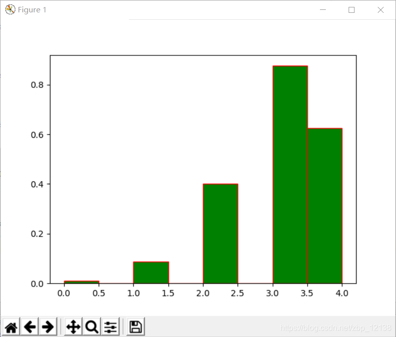
二项分布:
s_binomial = np.random.binomial(n=4,p=0.75,size=1000) #二项分布
plt.hist(s_binomial,color='g',edgecolor='r',bins=8, normed=True)
plt.show()
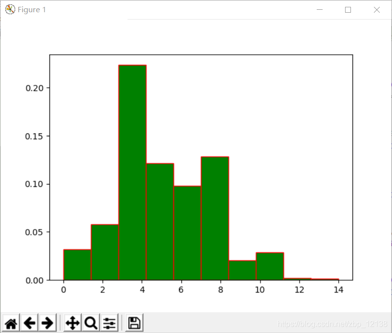
泊松分布:
s_poisson = np.random.poisson(lam=5,size=1000) #泊松分布
plt.hist(s_poisson,color='g',edgecolor='r',bins=10, normed=True)
plt.show()
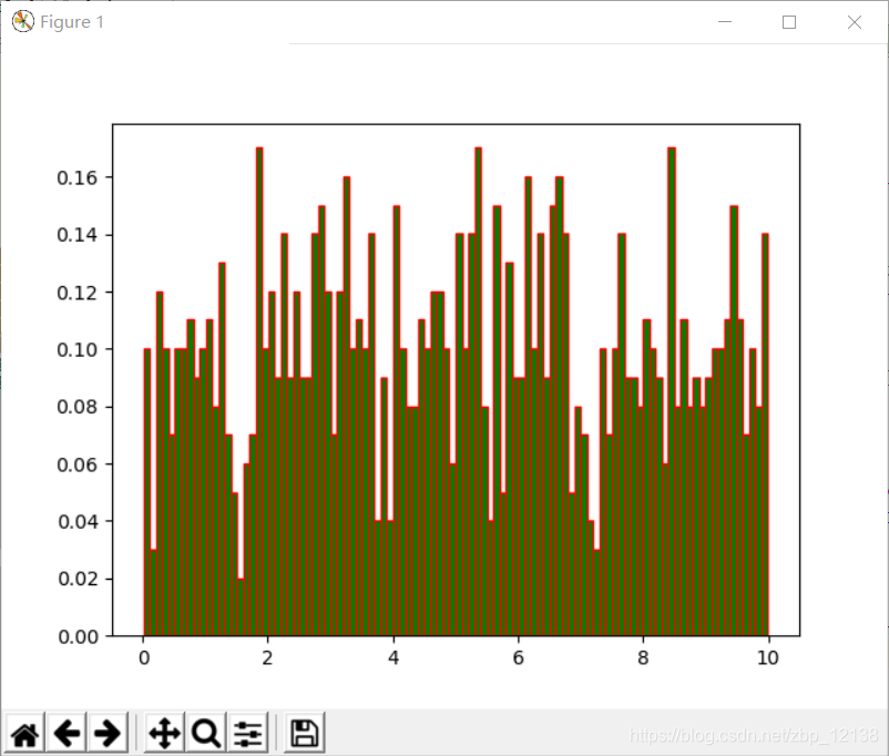
均匀分布:
s_uniform = np.random.uniform(low=0,high=10,size=1000)  #均匀分布
plt.hist(s_uniform,color='g',edgecolor='r',bins=100, normed=True)
plt.show()
指数分布:
s_exponential = np.random.exponential(scale=0.125,size=1000)  #指数分布
plt.hist(s_exponential,color='g',edgecolor='r',bins=100, normed=True)
plt.show()

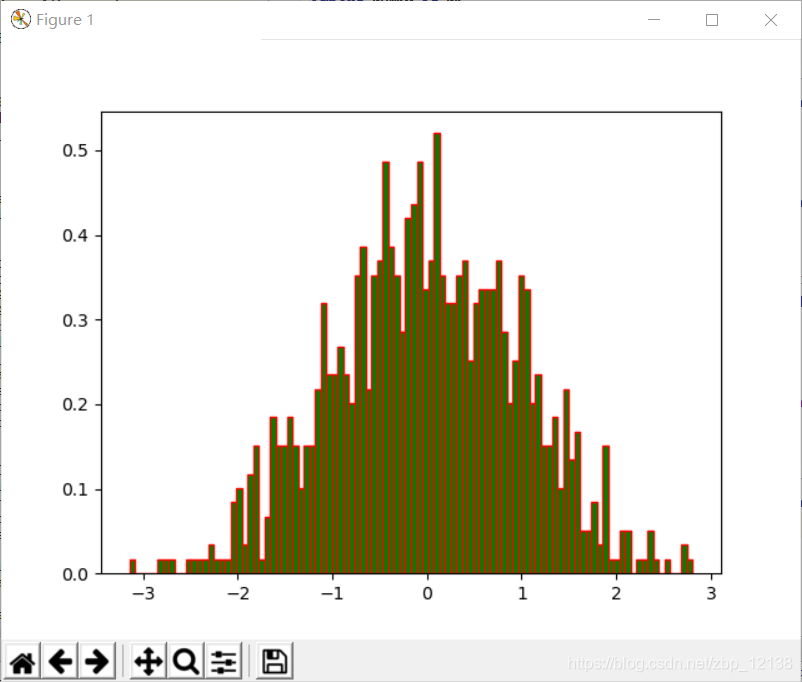
正态分布:
s_normal = np.random.normal(loc=0,scale=1,size=1000)  #正态分布
plt.hist(s_normal,color='g',edgecolor='r',bins=100, normed=True)
plt.show()