抛硬币问题可能是贝叶斯推断中最基础的一个入门问题,该问题简单来说就是对一枚硬币出现正面朝上的概率θ进行估计。不同于MLE, MAP等估计方法求出的是一个估计值,贝叶斯分析求出的是一个后验分布(用贝叶斯公式)。
θ的先验通常选用beta分布,n次观测正面朝上次数y的似然则可以用参数为n和θ二项分布来描述。用数学表达式描述如下θ ~ Beta(α, β),y~ Bin(n, p = θ).
这里顺便多说一下为什么先验用beta分布的原因:One of them is that the beta distribution is restricted to be between 0 and 1, in the same way our parameter θ is. Another reason is its versatility. As we can see in the preceding figure, the distribution adopts several shapes, including a uniform distribution, Gaussian-like distributions, U-like distributions, and so on. A third reason is that the beta distribution is the conjugate prior of the binomial distribution (which we are using as the likelihood). A conjugate prior of a likelihood is a prior that, when used in combination with the given likelihood, returns a posterior with the same functional form as the prior. Untwisting the tongue, every time we use a beta distribution as prior and a binomial distribution as likelihood, we will get a beta as a posterior. 也就是说在这里,后验分布可以直接求出解析解 θ|y ~ Beta(α_prior + α,β_prior + N -y). 当然,使用现代计算方法(如MCMC采样),我们进行贝叶斯推断时无需考虑是否使用共轭先验。(we can use modern computational methods to solve Bayesian problems whether we choose conjugate priors or not.)
代码如下:
# -*- coding: utf-8 -*-
import pymc3 as pm
import numpy as np
import scipy.stats as stats
import matplotlib.pyplot as plt
if __name__ == "__main__":
np.random.seed(123)
n_experiments = 100
theta_real = 0.35 # unkwon value in a real experiment
alpha_prior = 1
beta_prior = 1
data = stats.bernoulli.rvs(p=theta_real, size=n_experiments)
data_sum = data.sum()
with pm.Model() as our_first_model:
# a priori
theta = pm.Beta('theta', alpha=1, beta=1)
# likelihood
y = pm.Bernoulli('y', p=theta, observed=data)
#y = pm.Binomial('theta',n=n_experimentos, p=theta, observed=sum(datos))
start = pm.find_MAP()
step = pm.Metropolis()
trace = pm.sample(2000, step=step, start=start, nchains = 1)
burnin = 0 # no burnin
chain = trace[burnin:]
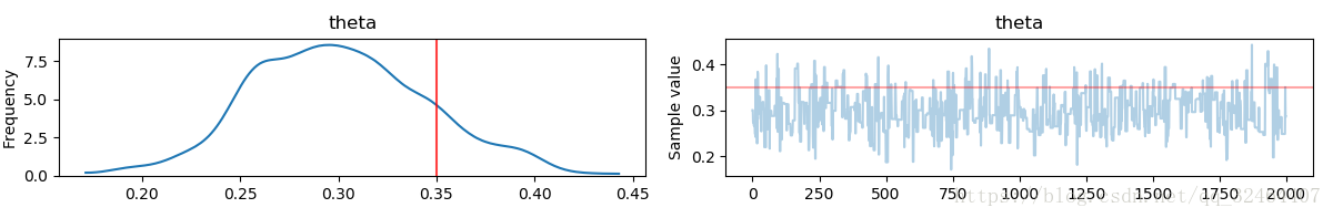
pm.traceplot(chain, lines={'theta':theta_real});
plt.figure()
x = np.linspace(.2, .6, 1000)
func = stats.beta(a =alpha_prior+data_sum, b=beta_prior+n_experiments-data_sum)
y = func.pdf(x)
plt.plot(x, y, 'r-', lw=3, label='True distribution')
plt.hist(chain['theta'], bins=30, normed=True, label='Estimated posterior distribution')
输出(采样轨迹和推断出的后验分布直方图):