
一个栗子
 1 >>>import numpy as np
 2
 3 >>>a = np.arange(15).reshape(3, 5)
 4
 5 >>>a
 6
 7 array([[ 0,    1,    2,    3,    4],
 8
 9 [5, 6, 7, 8, 9], [10, 11, 12, 13, 14]])
10 >>>a.shape
11
12 (3, 5)
13
14 >>>a.ndim  # 数组轴的个数,在python的世界中,轴的个数被称作秩
15
16 2
17
18 >>>a.dtype.name
19
20 'int64'
21
22 >>>a.itemsize  # 数组中每个元素的字节大小。
23
24 8
25
26 >>>a.size
27
28 15
29
30 >>>type(a)
31
32 <type 'numpy.ndarray'>
33
34 >>>b = np.array([6, 7, 8])
35
36 >>>b
37
38 array([6, 7, 8])
39
40 >>>type(b)
41
42 <type 'numpy.ndarray'>
基本数据类型
Numpy 常见的基本数据类型如下:
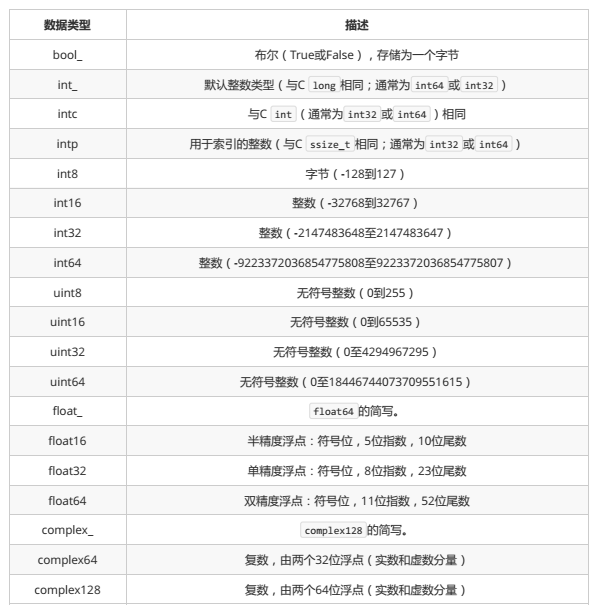
以上这些数据类型都可以通过 np.bool_ 、 np.float32 等方式访问。
这些类型都可以在创建 ndarray 时通过参数 dtype 来指定。
类型转换
要转换数组的类型,请使用.astype()方法(首选)或类型本身作为函数。
 1 >>>a
 2
 3 array([ 0.,    1.,    2.])
 4
 5 >>>a.astype(np.bool_)
 6
 7 array([False,    True,    True], dtype=bool)
 8
 9 >>>np.bool_(a)
10
11 array([False,    True,    True], dtype=bool)
创建矩阵(采用ndarray对象)
对于Python中的numpy模块,一般用其提供的ndarray对象。创建一个ndarray对象很简单,只要将一个list作为参数即可。例如:
 1 >>>import numpy as np
 2
 3 #创建一维的narray对象
 4
 5 >>>a = np.array([2,3,4])
 6
 7 >>>a
 8
 9 array([2, 3, 4])
10
11 >>>a.dtype dtype('int64')
12 # 浮点类型
13
14 >>>b = np.array([1.2, 3.5, 5.1])
15
16 >>>b.dtype
17
18 dtype('float64')
19
20 #创建二维的narray对象
21
22 >>>a2 = np.array([[1,2,3,4,5],[6,7,8,9,10]])
23
24 >>>b = np.array([(1.5,2,3), (4,5,6)])  # 使用的是元组
25
26 >>>b
27
28 array([[ 1.5,    2. ,    3. ],
29
30 [4. ,  5. ,  6. ]])
31
32 #The type of the array can also be explicitly specified at creation time:
33
34 >>> c = np.array( [ [1,2], [3,4] ], dtype=complex )
35
36 >>> c
37
38 array([[ 1.+0.j,  2.+0.j],
39
40 [3.+0.j,  4.+0.j]])
矩阵行数列数(二维情况)
1 import numpy as np
2
3 a = np.array([[1,2,3,4,5],[6,7,8,9,10]])
4
5 print(a.shape) #结果返回一个tuple元组 (2, 5) 2行,5列 print(a.shape[0]) #获得行数,返回 2 print(a.shape[1]) #获得列数,返回 5
矩阵的截取
按行列截取
矩阵的截取和list相同,可以通过[ ](方括号)来截取
1 import numpy as np
2
3 a = np.array([[1,2,3,4,5],[6,7,8,9,10]])
4
5 print(a[0:1]) #截取第一行,返回 [[1 2 3 4 5]]
6
7 print(a[1,2:5]) #截取第二行,第三、四、五列,返回 [8 9 10]
8
9 print(a[1,:]) #截取第二行,返回 [ 6    7    8    9 10]
按条件截取
 1 import numpy as np
 2
 3 a = np.array([[1,2,3,4,5],[6,7,8,9,10]])
 4
 5 b = a[a>6] # 截取矩阵a中大于6的元素,返回的是一维数组 print(b) # 返回 [ 7 8 9 10]
 6
 7 #其实布尔语句首先生成一个布尔矩阵,将布尔矩阵传入[](方括号)实现截取 print(a>6)
 8
 9 #返回
10
11 [[False False False False False]
12
13 [False    True    True    True    True]]
按条件截取应用较多的是对矩阵中满足一定条件的元素变成特定的值。 例如将矩阵中大于6的元素变成0。
import numpy as np
a = np.array([[1,2,3,4,5],[6,7,8,9,10]])
print(a)
#开始矩阵为
[[ 1 2 3 4 5]
[6 7 8 9 10]]
>>>a[a>6] = 0
print(a)
#大于6清零后矩阵为
[[1 2 3 4 5]
[6 0 0 0 0]]
>>>y
array([[ 0, 1, 2, 3, 4, 5, 6],
[7, 8, 9, 10, 11, 12, 13], [14, 15, 16, 17, 18, 19, 20], [21, 22, 23, 24, 25, 26, 27], [28, 29, 30, 31, 32, 33, 34]])
>>>b = y > 20
>>>y[b]
array([21, 22, 23, 24, 25, 26, 27, 28, 29, 30, 31, 32, 33, 34])
Stacking together different arrays
矩阵的合并可以通过numpy中的hstack方法和vstack方法实现:
>>>a = np.floor(10*np.random.random((2,2)))
>>>a
array([[ 8., 8.],
[0., 0.]])
>>>b = np.floor(10*np.random.random((2,2)))
>>>b
array([[ 1., 8.],
[0., 4.]])
>>>np.vstack((a,b)) array([[ 8., 8.],
[0., 0.],
[1., 8.],
[0., 4.]])
>>>np.hstack((a,b))
array([[ 8., 8., 1., 8.],
[ 0., 0., 0., 4.]])
矩阵的合并也可以通过concatenate方法。
np.concatenate( (a1,a2), axis=0 ) 等价于 np.vstack( (a1,a2) )
np.concatenate( (a1,a2), axis=1 ) 等价于 np.hstack( (a1,a2) )
通过函数创建矩阵
arange
import numpy as np
a = np.arange(10) # 默认从0开始到10(不包括10),步长为1 print(a) # 返回 [0 1 2 3 4 5 6 7 8 9]
a1 = np.arange(5,10) # 从5开始到10(不包括10),步长为1 print(a1) # 返回 [5 6 7 8 9]
a2 = np.arange(5,20,2) # 从5开始到20(不包括20),步长为2 print(a2) # 返回 [ 5 7 9 11 13 15 17 19]
linspace / logspace
import numpy as np
# 类似于matlab
a = np.linspace(0,10,7) # 生成首位是0,末位是10,含7个数的等差数列 print(a)
#结果
[ 0. 1.66666667 3.33333333 5. 6.66666667 8.33333333 10. ]
>>>a = np.ones(3, dtype=np.int32) # 范围在‐2147483648‐‐‐2147483647
>>>b = np.linspace(0,pi,3)
>>>b.dtype.name
'float64'
>>>c = a+b
>>>c
array([ 1. , 2.57079633, 4.14159265])
>>>c.dtype.name 'float64'
>>>d = np.exp(c*1j)
>>>d
array([ 0.54030231+0.84147098j, ‐0.84147098+0.54030231j, ‐0.54030231‐0.84147098j])
>>>d.dtype.name 'complex128'
ones、zeros、eye、empty
ones创建全1矩阵 ,zeros创建全0矩阵 ,eye创建单位矩阵 ,empty创建空矩阵(实际有值)
import numpy as np
a_ones = np.ones((3,4)) # 创建3*4的全1矩阵
print(a_ones)
#结果
[[ 1. 1. 1. 1.]
[1. 1. 1. 1.]
[1. 1. 1. 1.]]
>>> np.ones((2,3,4), dtype=np.int16 ) # dtype can also be specified array([[[ 1, 1, 1, 1],
[1, 1, 1, 1],
[1, 1, 1, 1]],
[[ 1, 1, 1, 1],
[1, 1, 1, 1],
[1, 1, 1, 1]]], dtype=int16) # Int16在‐32768 到 +32767之间
a_zeros = np.zeros((3,4)) # 创建3*4的全0矩阵
print(a_zeros)
#结果
[[ 0. 0. 0. 0.]
[0. 0. 0. 0.]
[0. 0. 0. 0.]]
a_eye = np.eye(3) # 创建3阶单位矩阵
print(a_eye)
#结果
[[ 1. 0. 0.]
[0. 1. 0.]
[0. 0. 1.]]
a_empty = np.empty((3,4)) # 创建3*4的空矩阵
print(a_empty)
#结果
[[ 1.78006111e‐306 ‐3.13259416e‐294 4.71524461e‐309 1.94927842e+289]
[ 2.10230387e‐309 5.42870216e+294 6.73606381e‐310 3.82265219e‐297]
[ 6.24242356e‐309 1.07034394e‐296 2.12687797e+183 6.88703165e‐315]]
#有些矩阵太大,如果不想省略中间部分,通过set_printoptions来强制NumPy打印所有数据。
>>> np.set_printoptions(threshold='nan')
fromstring
fromstring()方法可以将字符串转化成ndarray对象,需要将字符串数字化时这个方法比较有用,可以获得字符串的ascii码序列。
import numpy as np
a = "abcdef"
b = np.fromstring(a,dtype=np.int8) # 因为一个字符为8位,所以指定dtype为np.int8
#一个字母(例如:a、#、!之类的)用了1个字节来存储,1byte 即8位. print(b) # 返回 [ 97 98 99 100 101 102]
random
>>>a = np.random.random((2,3)) # 产生2行,3列的随机矩阵
>>>a
array([[ 0.18626021, 0.34556073, 0.39676747],
[0.53881673, 0.41919451, 0.6852195 ]])
fromfunction
fromfunction()方法可以根据矩阵的行号列号生成矩阵的元素。 例如创建一个矩阵,矩阵中的每个元素都为行号和列号的和。
import numpy as np
def func(i,j):
return i+j
a = np.fromfunction(func,(5,6))
#第一个参数为指定函数,第二个参数为列表list或元组tuple,说明矩阵的大小 print(a)
#返回
[[ 0. 1. 2. 3. 4. 5.]
[1. 2. 3. 4. 5. 6.]
[2. 3. 4. 5. 6. 7.]
[3. 4. 5. 6. 7. 8.]
[4. 5. 6. 7. 8. 9.]]
#注意这里行号的列号都是从0开始的
矩阵的运算
常用矩阵运算符
Numpy中的ndarray对象重载了许多运算符,使用这些运算符可以完成矩阵间对应元素的运算。
运算符 说明
+ 矩阵对应元素相加
- 矩阵对应元素相减
* 矩阵对应元素相乘
/ 矩阵对应元素相除,如果都是整数则取商
% 矩阵对应元素相除后取余数
** 矩阵每个元素都取n次方,如**2:每个元素都取平方
import numpy as np
a1 = np.array([[4,5,6],[1,2,3]])
a2 = np.array([[6,5,4],[3,2,1]])
print(a1+a2) # 相加
#结果
[[10 10 10]
[4 4 4]]
print(a1/a2) # 整数相除取商
#结果
[[0 1 1] [0 1 3]]
print(a1%a2) # 相除取余数
#结果
[[4 0 2] [1 0 0]]
常用矩阵函数
同样地,numpy中也定义了许多函数,使用这些函数可以将函数作用于矩阵中的每个元素。 表格中默认导入了
numpy模块,即 import numpy as np 。a为ndarray对象。
常用矩阵函数 说明
np.sin(a) 对矩阵a中每个元素取正弦,sin(x)
np.cos(a) 对矩阵a中每个元素取余弦,cos(x)
np.tan(a) 对矩阵a中每个元素取正切,tan(x)
np.arcsin(a) 对矩阵a中每个元素取反正弦,arcsin(x)
np.arccos(a) 对矩阵a中每个元素取反余弦,arccos(x)
np.arctan(a) 对矩阵a中每个元素取反正切,arctan(x)
np.exp(a) 对矩阵a中每个元素取指数函数,ex
np.sqrt(a) 对矩阵a中每个元素开根号
当矩阵中的元素不在函数定义域范围内,会产生RuntimeWarning,结果为nan(not a number)
矩阵乘法(点乘)
矩阵乘法必须满足矩阵乘法的条件,即第一个矩阵的列数等于第二个矩阵的行数。 矩阵乘法的函数为 dot 。
import numpy as np
a1 = np.array([[1,2,3],[4,5,6]]) # a1为2*3矩阵
a2 = np.array([[1,2],[3,4],[5,6]]) # a2为3*2矩阵
print(a1.shape[1]==a2.shape[0]) # True, 满足矩阵乘法条件 print(a1.dot(a2))
#a1.dot(a2)相当于matlab中的a1*a2
#而Python中的a1*a2相当于matlab中的a1.*a2
#结果
[[22 28]
[49 64]]
矩阵的转置 a.T
import numpy as np
a = np.array([[1,2,3],[4,5,6]])
print(a.transpose())
#结果
[[1 4] [2 5] [3 6]]
矩阵的转置还有更简单的方法,就是a.T。
import numpy as np
a = np.array([[1,2,3],[4,5,6]])
print(a.T)
#结果
[[1 4] [2 5] [3 6]]
矩阵的逆
设A是数域上的一个n阶方阵,若在相同数域上存在另一个n阶矩阵B,使得: AB=BA=E。 则我们称B是A的逆矩阵,而A则被称为可逆矩阵。E是单位矩阵。
求矩阵的逆需要先导入 numpy.linalg ,用 linalg 的 inv 函数来求逆。矩阵求逆的条件是矩阵应该是方阵。
import numpy as np
import numpy.linalg as lg
a = np.array([[1,2,3],[4,5,6],[7,8,9]])
print(lg.inv(a))
#结果
[[ ‐4.50359963e+15 9.00719925e+15 ‐4.50359963e+15]
[ 9.00719925e+15 ‐1.80143985e+16 9.00719925e+15]
[ ‐4.50359963e+15 9.00719925e+15 ‐4.50359963e+15]]
a = np.eye(3) # 3阶单位矩阵
print(lg.inv(a)) # 单位矩阵的逆为他本身
#结果
[[ 1. 0. 0.]
[0. 1. 0.]
[0. 0. 1.]]
矩阵信息获取(如均值等)
最值
获得矩阵中元素最大最小值的函数分别是 max 和 min ,可以获得整个矩阵、行或列的最大最小值。
import numpy as np
a = np.array([[1,2,3],[4,5,6]])
print(a.max()) #获取整个矩阵的最大值 结果: 6
print(a.min()) #结果:1
#可以指定关键字参数axis来获得行最大(小)值或列最大(小)值
#axis=0 行方向最大(小)值,即获得每列的最大(小)值
#axis=1 列方向最大(小)值,即获得每行的最大(小)值
#例如
print(a.max(axis=0)) # 每列的最大值
# 结果为 [4 5 6]
print(a.max(axis=1)) # 每行的最大值
#结果为 [3 6]
#要想获得最大最小值元素所在的位置,可以通过argmax函数来获得 print(a.argmax(axis=1))
#结果为 [2 2]
平均值
获得矩阵中元素的平均值可以通过函数 mean() 。同样地,可以获得整个矩阵、行或列的平均值。
import numpy as np
a = np.array([[1,2,3],[4,5,6]])
print(a.mean()) #结果为: 3.5
#同样地,可以通过关键字axis参数指定沿哪个方向获取平均值 print(a.mean(axis=0)) # 结果 [ 2.5 3.5 4.5] print(a.mean(axis=1)) # 结果 [ 2. 5.]
方差
方差的函数为 var() ,方差函数 var() 相当于函数 mean(abs(x - x.mean())**2) ,其中x为矩阵。
import numpy as np
a = np.array([[1,2,3],[4,5,6]])
print(a.var()) # 结果 2.91666666667
print(a.var(axis=0)) # 结果 [ 2.25 2.25 2.25]
print(a.var(axis=1)) # 结果 [ 0.66666667 0.66666667]
标准差
标准差的函数为 std() 。 std() 相当于 sqrt(mean(abs(x - x.mean())**2)) ,或相当于 sqrt(x.var()) 。
import numpy as np
a = np.array([[1,2,3],[4,5,6]])
print(a.std()) # 结果 1.70782512766
print(a.std(axis=0)) # 结果 [ 1.5 1.5 1.5]
print(a.std(axis=1)) # 结果 [ 0.81649658 0.81649658]
中值
中值指的是将序列按大小顺序排列后,排在中间的那个值,如果有偶数个数,则是排在中间两个数的平均值。中值
的函数是median(),调用方法为numpy.median(x,[axis]),axis可指定轴方向,默认axis=None,对所有数取中值。
import numpy as np
x = np.array([[1,2,3],[4,5,6]])
print(np.median(x)) # 对所有数取中值
#结果
3.5
print(np.median(x,axis=0)) # 沿第一维方向取中值
#结果
[2.5 3.5 4.5]
print(np.median(x,axis=1)) # 沿第二维方向取中值
#结果
[2. 5.]
求和
矩阵求和的函数是sum(),可以对行,列,或整个矩阵求和
import numpy as np
a = np.array([[1,2,3],[4,5,6]])
print(a.sum()) # 对整个矩阵求和
#结果 21
print(a.sum(axis=0)) # 对列方向求和
# 结果 [5 7 9]
print(a.sum(axis=1)) # 对行方向求和
# 结果 [ 6 15]
累积和
某位置累积和指的是该位置之前(包括该位置)所有元素的和。例如序列[1,2,3,4,5],其累计和为[1,3,6,10,15],即第一个元素为1,第二个元素为1+2=3,……,第五个元素为1+2+3+4+5=15。矩阵求累积和的函数是cumsum(),可以对行,列,或整个矩阵求累积和。
import numpy as np
a = np.array([[1,2,3],[4,5,6]])
print(a.cumsum()) # 对整个矩阵求累积和
# 结果 [ 1 3 6 10 15 21]
print(a.cumsum(axis=0)) # 对列方向求累积和
#结果
[[1 2 3] [5 7 9]]
print( a.cumsum(axis=1)) # 对行方向求累积和
#结果
[[ 1 3 6]
[4 9 15]]
极差
>>>import numpy as np
>>>a = np.arange(10)
>>>a.ptp()
#结果是
9
百分位数
numpy.percentile(a, q, axis)
序号 参数及描述
1. a 输入数组
2. q 要计算的百分位数,在 0 ~ 100 之间
3. axis 沿着它计算百分位数的轴
加权平均值
>>>data = range(1,5)
>>>data
[1, 2, 3, 4]
>>>np.average(data)
2.5
>>>np.average(range(1,11), weights=range(10,0,‐1))
4.0
>>>data = np.arange(6).reshape((3,2))
>>>data
array([[0, 1],
[2, 3],
[4, 5]])
>>>np.average(data, axis=1, weights=[1./4, 3./4]) array([ 0.75, 2.75, 4.75])
>>>np.average(data, weights=[1./4, 3./4]) Traceback (most recent call last):
...
TypeError: Axis must be specified when shapes of a and weights differ.
Shape Manipulation
Changing the shape of an array
>>>a = np.floor(10*np.random.random((3,4)))
>>>a
array([[ 2., 8., 0., 6.],
[ 4., 5., 1., 1.],
[8., 9., 3., 6.]])
>>>a.shape
(3, 4)
数组的形状可以用以下方式改变。Note that the following three commands all return a modified array, but do not change the original array:
>>>a.ravel() # returns the array, flattened
array([ 2., 8., 0., 6., 4., 5., 1., 1., 8., 9., 3., 6.])
>>>a.reshape(6,2) # returns the array with a modified shape array([[ 2., 8.],
[0., 6.],
[4., 5.],
[1., 1.],
[8., 9.],
[3., 6.]])
>>>a.T # returns the array, transposed
array([[ 2., 4., 8.],
[8., 5., 9.],
[0., 1., 3.],
[6., 1., 6.]])
>>>a.T.shape
(4, 3)
>>>a.shape (3, 4)
The reshape function returns its argument with a modified shape, whereas the ndarray.resize method modifies the array itself:
>>> a
array([[ 2., 8., 0., 6.],
[ 4., 5., 1., 1.],
[8., 9., 3., 6.]])
>>>a.resize((2,6))
>>>a
array([[ 2., 8., 0., 6., 4., 5.],
[ 1., 1., 8., 9., 3., 6.]])
If a dimension is given as -1 in a reshaping operation, the other dimensions are automatically calculated:
>>>a.reshape(3,‐1)
array([[ 2., 8., 0., 6.],
[ 4., 5., 1., 1.],
[8., 9., 3., 6.]])
Splitting one array into several smaller ones
Using hsplit , you can split an array along its horizontal axis, either by specifying the number of equally shaped arrays to return, or by specifying the columns after which the division should occur:
>>>a = np.floor(10*np.random.random((2,12)))
>>>a
array([[ 9., 5., 6., 3., 6., 8., 0., 7., 9., 7., 2., 7.],
[ 1., 4., 9., 2., 2., 1., 0., 6., 2., 2., 4., 0.]])
>>> np.hsplit(a,3) # Split a into 3
[array([[ 9., 5., 6., 3.],
[ 1., 4., 9., 2.]]), array([[ 6., 8., 0., 7.],
[ 2., 1., 0., 6.]]), array([[ 9., 7., 2., 7.],
[ 2., 2., 4., 0.]])]
Copies and Views
When operating and manipulating arrays, their data is sometimes copied into a new array and sometimes not. This is often a source of confusion for beginners. There are three cases:
No Copy At All(完全不复制)
a= b,改变b就相当于改变a,或者相反。
>>>a = np.arange(12)
>>> b = a # no new object is created
>>> b is a # a and b are two names for the same ndarray object
True
>>>b.shape = 3,4# changes the shape of a
>>>a.shape
(3, 4)
View or Shallow Copy(视图或浅复制)
Different array objects can share the same data. The view method creates a new array object that looks at the same data.
>>>c = a.view()
>>>c is a False
>>> c.base is a # c is a view of the data owned by a
True
>>> c.flags.owndata # c并不拥有数据
False
>>>
>>> c.shape = 2,6 # a's shape doesn't change
>>> a.shape
(3, 4)
>>> c[0,4] = 1234 # a's data changes a 的数据也会变
>>> a
array([[ 0, 1, 2, 3],
[1234, 5, 6, 7],
[ 8, 9, 10, 11]])
Slicing an array returns a view of it:
>>>s = a[:,1:3] # spaces added for clarity; could also be written "s = a[:,1:3]"
>>>s[:] = 10# s[:] is a view of s. Note the difference between s=10 and s[:]=10
>>>a
array([[ 0, 10, 10, 3],
[1234, 10, 10, 7],
[8, 10, 10, 11]])
Deep Copy(深复制)
The copy method makes a complete copy of the array and its data.
>>> d = a.copy() # a new array object with new data is created
>>>d is a False
# d没有和a共享任何数据
>>> d.base is a # d doesn't share anything with a
False
>>>d[0,0] = 9999
>>>a
array([[ 0, 10, 10, 3],
[1234, 10, 10, 7],
[8, 10, 10, 11]])
numpy 关于 copy 有三种情况,完全不复制、视图(view)或者叫浅复制( shadow copy )和深复制( deep
copy )。而 b = a[:] 就属于第二种,即视图,这本质上是一种切片操作( slicing ),所有的切片操作返回的
都是视图。具体来说, b = a[:] 会创建一个新的对象 b (所以说 id 和 a 不一样),但是 b 的数据完全来自于 a ,和 a 保持完全一致,换句话说,b的数据完全由a保管,他们两个的数据变化是一致的,可以看下面的示例:
a = np.arange(4) # array([0, 1, 2, 3])
b = a[:] # array([0, 1, 2, 3])
b.flags.owndata # 返回 False,b 并不保管数据
a.flags.owndata # 返回 True,数据由 a 保管
#改变 a 同时也影响到 b
a[‐1] = 10 # array([0, 1, 2, 10])
b# array([0, 1, 2, 10])
#改变 b 同时也影响到 a
b[0] = 10 # array([10, 1, 2, 10])
a# array([10, 1, 2, 10])
b = a 和 b = a[:] 的差别就在于后者会创建新的对象,前者不会。两种方式都会导致 a 和 b 的数据相互影响。要想不让 a 的改动影响到 b ,可以使用深复制: unique_b = a.copy()
曼德勃罗
import numpy as np
import matplotlib.pyplot as plt
def mandelbrot( h,w, maxit=20 ):
"""Returns an image of the Mandelbrot fractal of size (h,w)."""
y,x = np.ogrid[ ‐1.4:1.4:h*1j, ‐2:0.8:w*1j ]
c = x+y*1j
z = c
divtime = maxit + np.zeros(z.shape, dtype=int)
for i in range(maxit):
z = z**2 + c
diverge = z*np.conj(z) > 2**2
div_now = diverge & (divtime==maxit)
divtime[div_now] = i
# who is diverging
# who is diverging now
# note when
z[diverge] = 2 # avoid diverging too much
return divtime
plt.imshow(mandelbrot(400,400))
plt.show()