


# the aboving figure represents a sample, each loop represents a new sample travel which may lead the weigtht vector's update
# x1: with many features or a feature Vector
# x2: with many features or a feature Vector
import numpy as np
randomGenerator = np.random.RandomState(0)
weightVector = randomGenerator.normal(loc=0.0, scale=0.01, size=1+3)
weightVector
![]()
class Perceptron(object):
def __init__(self, eta =0.01, n_iter=10, random_state=1):
self.eta = eta #Learning rate (between 0.0 and 1.0)
self.n_iter = n_iter
self.random_state = random_state #Random number generator seed for random weight initialization.
def fit(self, X, y): #y:Target values. #X:shape = [n_samples, n_features]
rgen = np.random.RandomState(self.random_state)
#mu #sigma #n_features
self.w_ = rgen.normal(loc=0.0, scale=0.01, size=1+X.shape[1]) #1:self.w_[0]
#If all the weights are initialized to zero, the learning rate parameter
#eta affects only the scale of the weight vector,
self.errors_ = [] #Number of misclassifications (updates) in each epoch.
for _ in range(self.n_iter): #may have a new weightVector on each epoch/iteration
errors = 0
for xi, target in zip(X,y): #xi_sample,target_sample_label
#delta_weight_vector
update = self.eta * (target - self.predict(xi))
#updating the weights of features after evaluating each individual training sample,
self.w_[1:] += update * xi # xi_with featureVector * update
self.w_[0] += update
#print(self.w_)
errors += int(update !=0.0)
self.errors_.append(errors) #errors == all X_samples' error
return self
def net_input(self, X): # X_feature_vector * w^T
return np.dot(X, self.w_[1:]) + self.w_[0]
def predict(self, X): #X_feature_vector
return np.where(self.net_input(X) >= 0.0, 1, -1)
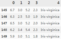
import pandas as pd
df = pd.read_csv('L:/MachineLearningInAction/machine_learning_databases/iris/iris.data', header=None)
df.tail()
import matplotlib.pyplot as plt
import numpy as np
# select setosa and versicolor
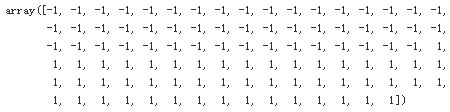
y = df.iloc[0:100, 4].values
y = np.where(y=='Iris-setosa', -1, 1)
y
# extract sepal length and peta length
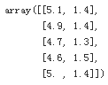
X = df.iloc[0:100, [0,2]].values
X[:5]
# plot data
plt.scatter(X[:50, 0], X[:50, 1], color='red', marker = 'o', label = 'setosa')
plt.scatter(X[50:100,0], X[50:100,1], color = 'blue', marker='x', label='versicolor')
plt.xlabel('sepal length [cm]')
plt.ylabel('petal length [cm]')
plt.legend(loc='upper left')
plt.show()

ppn = Perceptron(eta=0.1, n_iter=10)
ppn.fit(X,y)
plt.plot(range(1, len(ppn.errors_) + 1), ppn.errors_, marker='o')
plt.xlabel('Epochs')
plt.ylabel('Number of updates') # the changes of weightVector
plt.show()

from matplotlib.colors import ListedColormap
def plot_decision_regions(X, y, classifier, resolution =0.02):
#setup marker generator and color map
markerTuple =('s', 'x', 'o', '^', 'v')
colorTuple = ('red', 'blue', 'lightgreen', 'gray', 'cyan')
# take 'red' and 'blue'
cmap = ListedColormap(colorTuple[:len(np.unique(y))]) #从颜色列表生成的颜色映射对象
#plot the decision surface
x1_min, x1_max = X[:,0].min()-1, X[:,0].max()+1 #feature 0
x2_min, x2_max = X[:,1].min()-1, X[:,1].max()+1 #feature 2
#np.arange(x1_min, x1_max, resolution) : feature0 array({min-1, ..., max+1})
#np.arange(x2_min, x2_max, resolution) : feature2 array({min-1, ..., max+1})
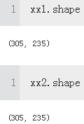
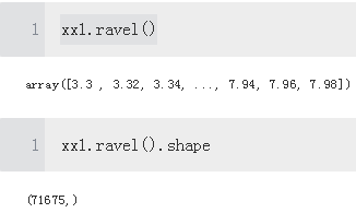
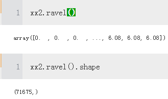
xx1, xx2 = np.meshgrid(np.arange(x1_min, x1_max, resolution), #columns = len(), repeated along row
np.arange(x2_min, x2_max, resolution)) #rows = len(), repeated along column
#xx1, xx2 are both two dimension array with same shape
#ravel(): Return a contiguous flattened array(one dimension)
#feature0 array({min-1, ..., max+1,..,min-1, ..., max+1})
#feature1 array({min-1, ..., max+1,..,min-1, ..., max+1})
#np.array([xx1.ravel(), xx2.ravel()]): two dimension array(features, samples)
Z = classifier.predict( np.array([xx1.ravel(), xx2.ravel()]).T ) #(samples, features)
Z = Z.reshape(xx1.shape) #one-to-one Z(xx1,xx2)
#axis,axis,height
plt.contourf(xx1, xx2, Z, alpha=0.3, cmap=cmap)
plt.xlim(xx1.min(), xx1.max()) #sepal length or x-axis or feature
plt.ylim(xx2.min(), xx2.max()) #petal length or y-axis or feature
#plot class samples
for idx, cl in enumerate(np.unique(y)):
#0 -1
#1 1
plt.scatter(x=X[y==cl, 0], #extracting
y=X[y==cl, 1],
alpha=0.8,
c=colorTuple[idx],
marker=markerTuple[idx],
label=cl,
edgecolor='black')
#ppn = Perceptron(eta=0.1, n_iter=10)
#ppn.fit(X,y)
plot_decision_regions(X, y, classifier=ppn)
plt.xlabel('sepal length [cm]')
plt.ylabel('petal length [cm]')
plt.legend(loc='upper left')
plt.show()

##########################################
Help for understanding


numpy.ravel(array_like):Return a contiguous flattened array.


##########################################
####################################################################################


#updating the weights based on the sum of the accumulated errors over all samples xi.
import pandas as pd
df = pd.read_csv('L:/MachineLearningInAction/machine_learning_databases/iris/iris.data', header=None)
df.head()

import matplotlib.pyplot as plt
import numpy as np
# select setosa and versicolor
y = df.iloc[0:100, 4].values
y = np.where(y=='Iris-setosa', -1, 1)
y
# extract sepal length and peta length
X = df.iloc[0:100, [0,2]].values
X[:5]

import numpy as np
class AdalineGD(object):
#Parameters
# eta: Learning rate (between 0.0 and 1.0)
# n_iter: Passes over the training dataset
# random_state: Random number generator seed for random weight
#Attributes
# w_ : 1d-array # weights after fitting
# cost_ : Sum-of-squares cost function value in each epoch
#random seed
def __init__(self, eta=0.01, n_iter=50, random_state=1):
self.eta = eta
self.n_iter = n_iter
self.random_state = random_state
def net_input(self, X): #intercept
return np.dot(X, self.w_[1:]) + self.w_[0] # X_features * w^T # result_single column matrix
def activation(self, X):
#Computer linear activation
return X
def fit(self, X, y): #X_array = [n_samples, n_features]
#y: label =[n_samples]
rgen = np.random.RandomState(self.random_state) #1+ n_features
self.w_ = rgen.normal( loc=0.0, scale=0.01, size=1+X.shape[1] )
self.cost_ = []
for i in range(self.n_iter):
net_input = self.net_input(X) # single column matrix
output = self.activation(net_input) #single column matrix
errors = (y-output) # result_vertical #single column matrix #rows == number of X_samples
#feature_weight
self.w_[1:] += self.eta * X.T.dot(errors) # X.T (n_features, n_samples) #single column matrix#rows==numberOfFeatures
self.w_[0] += self.eta * errors.sum()
cost = (errors **2).sum() /2.0
self.cost_.append(cost)
return self
def predict(self, X):
return np.where( self.activation( self.net_input(X) )>=0.0, 1, -1 )
import matplotlib.pyplot as plt
fig, ax = plt.subplots(nrows = 1, ncols =2, figsize=(10,4))
ada1 = AdalineGD(n_iter =10, eta=0.01).fit(X,y)
ax[0].plot( range(1, len(ada1.cost_) +1), np.log10(ada1.cost_), marker='o' )
ax[0].set_xlabel('Epochs')
ax[0].set_ylabel('log(Sum-squared-error)')
ax[0].set_title('Adaline-Learning rate 0.01')
ada2 = AdalineGD(n_iter=10, eta=0.0001).fit(X,y)
ax[1].plot( range(1, len(ada2.cost_) +1), ada2.cost_, marker='o')
ax[1].set_xlabel('Epochs')
ax[1].set_ylabel('Sum_squared-error')
ax[1].set_title('Adaline - Learning rate 0.0001')
plt.show()

As we can see in the resulting cost-function plots, we encountered two different types of problem. The left chart shows what could happen if we choose a learning rate that is too large. Instead of minimizing the cost function, the error becomes larger in every epoch, because we overshoot the global minimum. On the other hand, we can see that the cost decreases on the right plot, but the chosen learning rate![]() is so small that the algorithm would require a very large number of epochs to converge to the global cost minimum
is so small that the algorithm would require a very large number of epochs to converge to the global cost minimum

Improving gradient descent through feature scaling


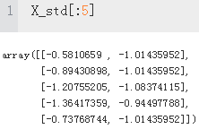
X_std = np.copy(X)
X_std[:,0] = (X[:,0] - X[:,0].mean()) / X[:,0].std()
X_std[:,1] = (X[:,1] - X[:,1].mean()) / X[:,1].std()
ada = AdalineGD(n_iter=15, eta=0.01)
ada.fit(X_std, y)
plot_decision_regions(X_std, y, classifier=ada)
plt.title('Adaline - Gradient Descent')
plt.xlabel('sepal length [standardized]')
plt.ylabel('petal length [standardized]')
plt.legend(loc='upper left')
plt.tight_layout()
plt.show()
plt.plot(range(1,len(ada.cost_) +1), ada.cost_, marker='o')
plt.xlabel('Epochs')
plt.ylabel('Sum-squared-error')
plt.show()


Large-scale machine learning and stochastic gradient descent
In the previous section, we learned how to minimize a cost function by taking a step in the opposite direction of a cost gradient that is calculated from the whole training set; this is why this approach is sometimes also referred to as batch gradient descent. Now imagine we have a very large dataset with millions of data points, which is not uncommon in many machine learning applications. Running batch gradient descent can be computationally quite costly in such scenarios since we need to reevaluate the whole training dataset each time we take one step towards the global minimum.
A popular alternative to the batch gradient descent algorithm is stochastic gradient descent, sometimes also called iterative or online gradient descent. Instead of updating the weights based on the sum of the accumulated errors over all samples

class AdalineSGD(object):
#Parameters
# eta: Learning rate (between 0.0 and 1.0)
# n_iter: Passes over the training dataset
# shuffle : bool (default: True) Shuffles training data every epoch if True to prevent cycles.
# random_state: Random number generator seed for random weight
#Attributes
# w_ : 1d-array # weights after fitting
# cost_ : Sum-of-squares cost function value in each epoch
#random seed
def __init__(self, eta=0.01, n_iter=10, shuffle=True, random_state=None):
self.eta = eta
self.n_iter = n_iter
self.w_initialized = False#############
self.shuffle = shuffle#############
self.random_state=random_state
def _initialize_weights(self, m):
self.rgen = np.random.RandomState(self.random_state)
self.w_ = self.rgen.normal(loc=0.0, scale=0.01, size=1+m) #numOfFeatures + 1
self.w_initialized = True
def activation(self, X):
return X
def net_input(self, X):
return np.dot(X, self.w_[1:]) + self.w_[0]
def _shuffle(self, X,y):
r=self.rgen.permutation(len(y)) #shuffle
return X[r], y[r] #selection or pick in order(r)
#via the permutation function in np.random, we generate a random sequence
#of unique numbers in the range 0 to 100. Those numbers can then be used as indices
#to shuffle our feature matrix and class label vector
def _update_weights(self, xi, target):
# Apply Adaline learning rule to update the weights
output = self.activation( self.net_input(xi) )
error = (target - output)
# VS self.w_[1:] += self.eta * X.T.dot(errors) # X.T (n_features, n_samples)
self.w_[1:] += self.eta * xi.dot(error)
self.w_[0] += self.eta * error
cost = 0.5 * error**2
return cost
def fit(self, X, y): # X : {array-like}, shape = [n_samples, n_features]
self._initialize_weights(X.shape[1])
self.cost_ = []
for i in range(self.n_iter):
if self.shuffle: #default True
X, y = self._shuffle(X,y)
cost = []
for xi, target in zip(X,y):
cost.append(self._update_weights(xi, target))
avg_cost = sum(cost) / len(y)
self.cost_.append(avg_cost)
return self
def partial_fit(self, X, y):
if not self.w_initialized:
self._initialize_weights(X.shape[1])
if y.ravel().shape[0] > 1:
for xi, target in zip(X,y):
self._update_weights(xi, target)
else:
self._update_weights(X,y)
return self
def predict(self, X):
return np.where(self.activation(self.net_input(X))>=0.0, 1, -1)
ada = AdalineSGD(n_iter=15, eta=0.01, random_state=1)
ada.fit(X_std, y)
plot_decision_regions(X_std, y, classifier=ada)
plt.title('Adaline - Stochastic Gradient Descent')
plt.xlabel('sepal length [standardized]')
plt.ylabel('petal length [standardized]')
plt.legend(loc='upper left')
plt.show()
plt.plot(range(1, len(ada.cost_)+1), ada.cost_, marker='o')
plt.xlabel('Epochs')
plt.ylabel('Average Cost')
plt.show()

As we can see, the average cost goes down pretty quickly, and the final decision
boundary after 15 epochs looks similar to the batch gradient descent Adaline. If we
want to update our model, for example, in an online learning scenario with streaming
data, we could simply call the partial_fit method on individual samples—for
instance ada.partial_fit(X_std[0, :], y[0]).
