引言
一直以来,卷积神经网络对人们来说都是一个黑箱,我们只知道它识别图片准确率很惊人,但是具体是怎么做到的,它究竟使用了什么特征来分辨图像,我们一无所知。无数的学者、研究人员都想弄清楚CNN内部运作的机制,甚至试图找到卷积神经网络和生物神经网络的联系。2013年,纽约大学的Matthew Zeiler和Rob Fergus的论文Visualizing and Understanding Convolutional Neural Networks用可视化的方法揭示了CNN的每一层识别出了什么特征,也揭开了CNN内部的神秘面纱。之后,也有越来越多的学者使用各种方法将CNN的每一层的激活值、filters等等可视化,让我们从各个方面了解到CNN内部的秘密。
分为两部分
- 可视化卷积神经网络提取的特征
- 可视化卷积神经网的
卷积神经网络提取的图像是什么特征
我们以ResNet50为例对每个卷积层提取的特征进行可视化。
首先读取网络结构和预训练参数:
from keras.applications.resnet50 import ResNet50
model = ResNet50(weights=None,
                 include_top=False,)
model.load_weights('resnet50_weights_tf_dim_ordering_tf_kernels_notop.h5')
model.summary()
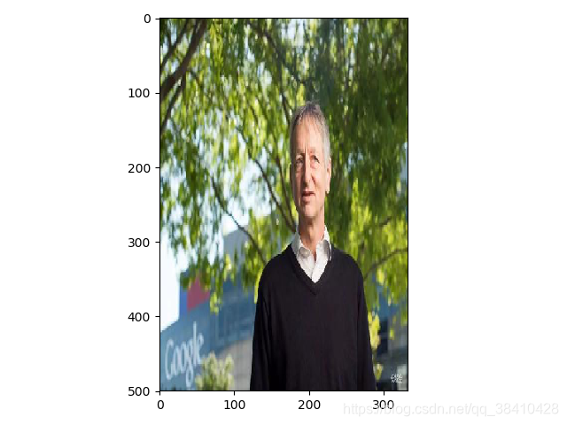
接下来读取一张图片,这里是以Hinton大佬图片为目标进行提取特征
from keras.preprocessing import image
import numpy as np
img_path = 'Hinton.jpg'
img = image.load_img(img_path, target_size=(500, 333))
img_tensor = image.img_to_array(img)
img_tensor = np.expand_dims(img_tensor, axis=0)
# Remember that the model was trained on inputs
# that were preprocessed in the following way:
img_tensor /= 255.

# Its shape is (1, 500, 333, 3)
print(img_tensor.shape)
结果:
(1, 500, 333, 3)
(1, 500, 333, 3)所代表的的含义是:
- 1,代表输入图片的个数,我们这里只输入了一个图片,所以是1;
- 500, 333,代表图片的大小;
- 3,代表该层有多少个filters(或者是通道数)。 所以,相当于我们的这一层输出了64张单通道图片。
图像展示
import matplotlib.pyplot as plt

plt.imshow(img_tensor[0])
plt.show()
获取ReSNet的层的输出
from keras import models
# 提取2-50层的特征
layer_outputs = [layer.output for layer in model.layers[2:51]]
# Creates a model that will return these outputs, given the model input:
activation_model = models.Model(inputs=model.input, outputs=layer_outputs)
为了提取要查看的特征图,我们将创建一个Keras模型,该模型将成批图像作为输入,并输出所有卷积和池化层的激活。 为此,我们将使用Keras类模型。 使用两个参数实例化一个Model:输入张量(或输入张量的列表)和输出张量(或输出张量的列表)。 生成的类是Keras模型,就像您熟悉的顺序模型一样,将指定的输入映射到指定的输出。 与顺序类不同,使Model类与众不同的是,它允许具有多个输出的模型。
# This will return a list of 5 Numpy arrays:
# one array per layer activation
activations = activation_model.predict(img_tensor)
这个activations里面,就装好了各层的所有的激活值。我们可以随便找一层的activation打印出来它的形状看看:
first_layer_activation = activations[0]
print(first_layer_activation.shape)
结果:
(1, 250, 167, 64)
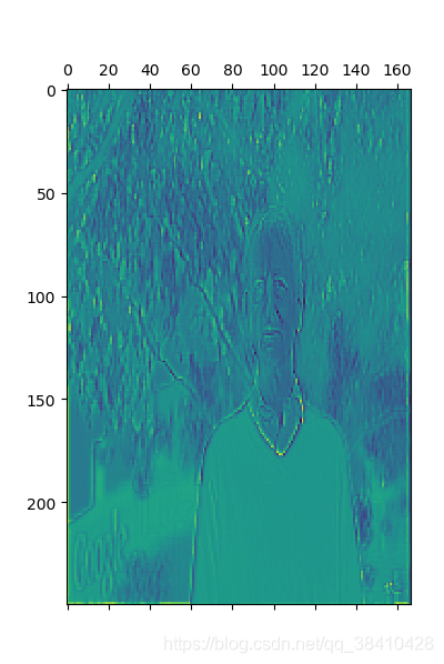
这是一个具有64个通道的250*167特征图,其中64代表着通道数。
可视化它的第三个通道:
import matplotlib.pyplot as plt
plt.matshow(first_layer_activation[0, :, :, 3], cmap='viridis')
plt.show()
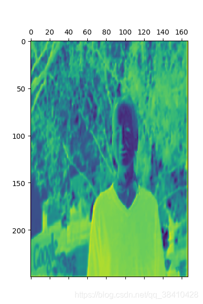
可视化它的第50个通道:
plt.matshow(first_layer_activation[0, :, :, 50], cmap='viridis')
plt.show()
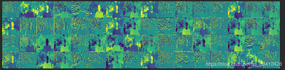
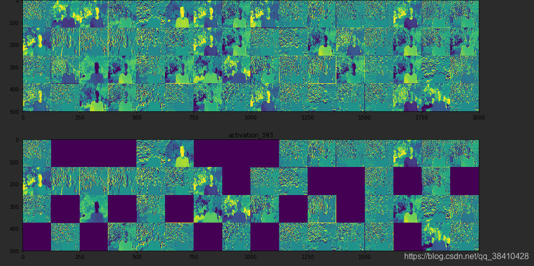
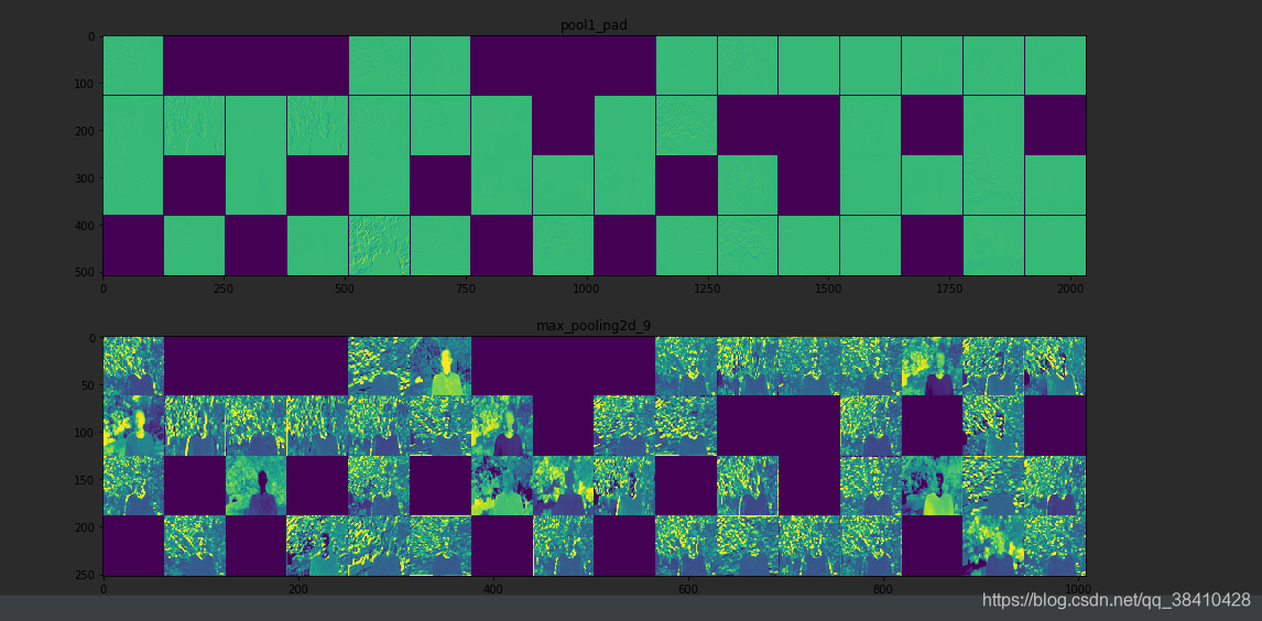
让我们对网络中所有激活进行完整的可视化绘制。 我们将提取并绘制每一个激活图中每个通道,并将结果堆叠在一个大图像张量中,通道并排堆叠。
import keras

# These are the names of the layers, so can have them as part of our plot
layer_names = []
for layer in model.layers[2:51]:
    layer_names.append(layer.name)

images_per_row = 16

# Now let's display our feature maps
for layer_name, layer_activation in zip(layer_names, activations):
    # This is the number of features in the feature map
    n_features = layer_activation.shape[-1]

    # The feature map has shape (1, size, size, n_features)
    size = layer_activation.shape[1]

    # We will tile the activation channels in this matrix
    n_cols = n_features // images_per_row
    display_grid = np.zeros((size * n_cols, images_per_row * size))

    # We'll tile each filter into this big horizontal grid
    for col in range(n_cols):
        for row in range(images_per_row):
            channel_image = layer_activation[0,
                                             :, :,
                                             col * images_per_row + row]
            # Post-process the feature to make it visually palatable
            channel_image -= channel_image.mean()
            channel_image /= channel_image.std()
            channel_image *= 64
            channel_image += 128
            channel_image = np.clip(channel_image, 0, 255).astype('uint8')
            display_grid[col * size : (col + 1) * size,
                         row * size : (row + 1) * size] = channel_image

    # Display the grid
    scale = 1. / size
    plt.figure(figsize=(scale * display_grid.shape[1],
                        scale * display_grid.shape[0]))
    plt.title(layer_name)
    plt.grid(False)
    plt.imshow(display_grid, aspect='auto', cmap='viridis')

plt.show()
等等。。。。。。
可视化卷积滤波器
这个过程很简单:我们将建立一个损失函数,使给定卷积层中给定滤波器的值最大化,然后我们将使用随机梯度下降来调整输入图像的值,以使该激活值最大化。 例如,这是在ImageNet上预训练的ResNet50网络的“ bn2a_branch2b ”层中激活过滤器0的损失:
from keras import backend as K
from keras.applications.resnet50 import ResNet50
model = ResNet50(weights=None,
                 include_top=False,)
model.load_weights('resnet50_weights_tf_dim_ordering_tf_kernels_notop.h5')
layer_name = 'bn2a_branch2b'
filter_index = 0
layer_output = model.get_layer(layer_name).output
loss = K.mean(layer_output[:, :, :, filter_index])
为了实现梯度下降,我们需要相对于模型输入的这种损失的梯度。 为此,我们将使用Keras后端模块附带的渐变函数:
# The call to `gradients` returns a list of tensors (of size 1 in this case)
# hence we only keep the first element -- which is a tensor.
grads = K.gradients(loss, model.input)[0]
要使梯度下降过程顺利进行的一个显而易见的技巧是通过将梯度张量除以其L2范数(张量中值的平方的平均值的平方根)来归一化。 这样可以确保对输入图像进行的更新幅度始终在同一范围内。
# We add 1e-5 before dividing so as to avoid accidentally dividing by 0.
grads /= (K.sqrt(K.mean(K.square(grads))) + 1e-5)
现在,在给定输入图像的情况下,我们需要一种方法来计算损耗张量和梯度张量的值。 我们可以定义一个Keras后端函数来做到这一点:iterate是一个接受Numpy张量(作为大小为1的张量的列表)并返回两个Numpy张量的列表的函数:损失值和梯度值。
在这一点上,我们可以定义一个Python循环来进行随机梯度下降:
# We start from a gray image with some noise
input_img_data = np.random.random((1, 150, 150, 3)) * 20 + 128.

# Run gradient ascent for 40 steps
step = 1.  # this is the magnitude of each gradient update
for i in range(40):
    # Compute the loss value and gradient value
    loss_value, grads_value = iterate([input_img_data])
    # Here we adjust the input image in the direction that maximizes the loss
    input_img_data += grads_value * step
生成的图像张量将是形状为(1,150,150,3)的浮点张量,其值不能为[0,255]内的整数。 因此,我们需要对该张量进行后处理,以将其转变为可显示的图像。 我们使用以下简单的实用程序功能来实现:
def deprocess_image(x):
    # normalize tensor: center on 0., ensure std is 0.1
    x -= x.mean()
    x /= (x.std() + 1e-5)
    x *= 0.1

    # clip to [0, 1]
    x += 0.5
    x = np.clip(x, 0, 1)

    # convert to RGB array
    x *= 255
    x = np.clip(x, 0, 255).astype('uint8')
    return x
现在我们拥有了所有内容,让我们将它们放到一个Python函数中,该函数接受一个图层名和一个过滤器索引作为输入,并返回一个有效的图像张量,该张量表示使指定过滤器的激活最大化的模式:
def generate_pattern(layer_name, filter_index, size=150):
    # Build a loss function that maximizes the activation
    # of the nth filter of the layer considered.
    layer_output = model.get_layer(layer_name).output
    loss = K.mean(layer_output[:, :, :, filter_index])

    # Compute the gradient of the input picture wrt this loss
    grads = K.gradients(loss, model.input)[0]

    # Normalization trick: we normalize the gradient
    grads /= (K.sqrt(K.mean(K.square(grads))) + 1e-5)

    # This function returns the loss and grads given the input picture
    iterate = K.function([model.input], [loss, grads])

    # We start from a gray image with some noise
    input_img_data = np.random.random((1, size, size, 3)) * 20 + 128.

    # Run gradient ascent for 40 steps
    step = 1.
    for i in range(40):
        loss_value, grads_value = iterate([input_img_data])
        input_img_data += grads_value * step

    img = input_img_data[0]
    return deprocess_image(img)
plt.imshow(generate_pattern('bn2a_branch2b', 0))
plt.show()

似乎bn2a_branch2b层中的过滤器0响应于圆点图案。
现在有趣的部分:我们可以开始可视化每一层中的每个滤镜。 为简单起见,我们将仅查看每层卷积块的前64个滤波器。 我们将输出排列在64x64滤镜模式的8x8网格上,每个滤镜模式之间有一些黑色边距。
for layer_name in ['conv1', 'res2a_branch2a', 'res2b_branch2a', 'res4e_branch2c']:
    size = 64
    margin = 5

    # This a empty (black) image where we will store our results.
    results = np.zeros((8 * size + 7 * margin, 8 * size + 7 * margin, 3))

    for i in range(8):  # iterate over the rows of our results grid
        for j in range(8):  # iterate over the columns of our results grid
            # Generate the pattern for filter `i + (j * 8)` in `layer_name`
            filter_img = generate_pattern(layer_name, i + (j * 8), size=size)

            # Put the result in the square `(i, j)` of the results grid
            horizontal_start = i * size + i * margin
            horizontal_end = horizontal_start + size
            vertical_start = j * size + j * margin
            vertical_end = vertical_start + size
            results[horizontal_start: horizontal_end, vertical_start: vertical_end, :] = filter_img

    # Display the results grid
    plt.figure(figsize=(20, 20))
    plt.imshow(results)
    plt.show()

