卷积神经网络的可视化（一）

卷积神经网络简单可视化

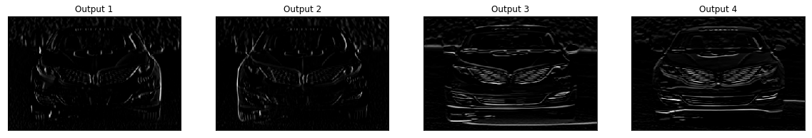
在本次练习中，我们将可视化卷积层 4 个过滤器的输出（即 feature maps）。

加载图像

import cv2
import matplotlib.pyplot as plt
%matplotlib inline

img_path = 'images/udacity_sdc.png'
bgr_img = cv2.imread(img_path)

gray_img = cv2.cvtColor(bgr_img, cv2.COLOR_BGR2GRAY)
gray_img = gray_img.astype("float32")/255

plt.imshow(gray_img, cmap='gray')
plt.show()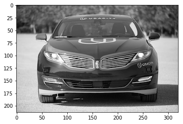

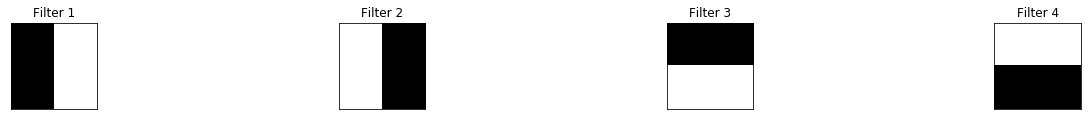
定义并可视化过滤器（卷积核）

import numpy as np

filter_vals = np.array([[-1, -1, 1, 1], [-1, -1, 1, 1], [-1, -1, 1, 1], [-1, -1, 1, 1]])

print('Filter shape: ', filter_vals.shape)

Filter shape:  (4, 4)

filter_1 = filter_vals
filter_2 = -filter_1
filter_3 = filter_1.T
filter_4 = -filter_3
filters = np.array([filter_1, filter_2, filter_3, filter_4])

print('Filter 1: \n', filter_1)

Filter 1: 
 [[-1 -1  1  1]
 [-1 -1  1  1]
 [-1 -1  1  1]
 [-1 -1  1  1]]

fig = plt.figure(figsize=(10, 5))
for i in range(4):
    ax = fig.add_subplot(1, 4, i+1, xticks=[], yticks=[])
    ax.imshow(filters[i], cmap='gray')
    ax.set_title('Filter %s' % str(i+1))
    width, height = filters[i].shape
    for x in range(width):
        for y in range(height):
            ax.annotate(str(filters[i][x][y]), xy=(y,x),
                       horizontalalignment='center',
                       verticalalignment='center',
                       color='white' if filters[i][x][y]<0 else 'black')

定义一个卷积层

初始化一个包含上面定义的过滤器（卷积核）的卷积层。下面并不是要训练这个卷积神经网络，而是通过过滤器初始化卷积层的权重，从而可以可视化，以看到图片经过一次前向传播后的变化。

import torch
import torch.nn as nn
import torch.nn.functional as F

class Net(nn.Module):
    def __init__(self, weight):
        super(Net, self).__init__()
        k_height, k_width = weight.shape[2:]
        self.conv = nn.Conv2d(1, 4, kernel_size=(k_height, k_width), bias=False)
        self.conv.weight = torch.nn.Parameter(weight)
        
    def forward(self, x):
        conv_x = self.conv(x)
        activated_x = F.relu(conv_x)
        
        return conv_x, activated_x

# filters 的大小为 4 4 4
# weight 的大小被增加为 4 1 4 4，1 的维度是针对输入的一个通道
weight = torch.from_numpy(filters).unsqueeze(1).type(torch.FloatTensor)
model = Net(weight)

print(filters.shape)
print(weight.shape)
print(model)

(4, 4, 4)
torch.Size([4, 1, 4, 4])
Net(
  (conv): Conv2d(1, 4, kernel_size=(4, 4), stride=(1, 1), bias=False)
)

可视化每个卷积核的输出

我们首先定义一个函数 viz_layer，以神经网络的一个层和卷积核的数量作为参数。在图像通过这个网络层的时候，这个方法可以可视化这一层的输出。

def viz_layer(layer, n_filters=4):
    fig = plt.figure(figsize=(20, 20))
    
    for i in range(n_filters):
        ax = fig.add_subplot(1, n_filters, i+1, xticks=[], yticks=[])
        ax.imshow(np.squeeze(layer[0,i].data.numpy()), cmap='gray')
        ax.set_title('Output %s' % str(i+1))

下面观察一层卷积层的输出，观察输出的可视化在 ReLU 激活函数前和激活函数后有什么区别。

plt.imshow(gray_img, cmap='gray')

fig = plt.figure(figsize=(12, 6))
fig.subplots_adjust(left=0, right=1.5, bottom=0.8, top=1, hspace=0.05, wspace=0.05)
for i in range(4):
    ax = fig.add_subplot(1, 4, i+1, xticks=[], yticks=[])
    ax.imshow(filters[i], cmap='gray')
    ax.set_title('Filter %s' % str(i+1))
    
# 为 gray img 添加 1 个 batch 维度，以及 1 个 channel 维度，并转化为 tensor
gray_img_tensor = torch.from_numpy(gray_img).unsqueeze(0).unsqueeze(1)
print(gray_img.shape)
print(gray_img_tensor.shape)
conv_layer, activated_layer = model(gray_img_tensor)
viz_layer(conv_layer)

(213, 320)
torch.Size([1, 1, 213, 320])

# after a ReLu is applied
# visualize the output of an activated conv layer
viz_layer(activated_layer)