1.内容回顾

关于Bezier曲线的定义和生成程序，请参考https://blog.csdn.net/iwanderu/article/details/103604863，本节内容会部分沿用上一节代码。

和曲线在空间的表示法一样，参数表示法来描述曲面更加方便，它的分类如下：

Bi-linear Patch
Ruled Patch
Coons Patch
Bi-cubic Patch
Hermite Patch
Coons Patch with tangents
Bezier Patch
B-Spline Patch
Non-Uniform Rational B-Splines (NURBS)
Other types of surfaces

本次讨论的内容是通过pyplot实现coons patch的绘制。
在这里插入图片描述
我们想描述的曲面为S(u,v),它由四个边界曲线P0,P1,Q0,Q1包围而成，注意，u和v的正方向为向上和向右为正，这个细节十分重要，因为绘图的时候使用一系列的点，放在array数组中来对应计算的，如果顺序错了，绘制的曲线就是错的。Coons Patch的参数化表达式如下：
在这里插入图片描述

其中alpha和beta是blending function，他们能调节曲面的起伏和光滑程度。默认alpha = 1 - u(对应上图的alpha0)， belta = 1 - v(对应上图的alpha1)，u和v分别是两个方向的坐标，注意他们的取值范围是0-1之间的，包括0和1.编程实现的基础就是这个公式。

2.题目描述

Based on your programming lab of curves, you are required in this lab to define and display Coons patches with different alpha(u) and belta(v) blending functions. You program should have the following functionalities.

(1) The user can define the four boundary curves of the Coons patch. The format of the curves is Bezier. For your convenience, you can assume that the number of control points of any Bezier curve is 6.

(2) You should allow the user to define different alpha(u) and belta(v). One suggestion is that you can define the alpha(u) (and belta(v)) as a Bezier curve with its two end control points on (0, 1) and (1, 0) respectively. For your convenience, you can fix the degree to 3 (i.e., 4 control points).

(3) Your program should be able to display the Coons patch by sampling the iso-curves and drawing their linear segments.

Note: when your program is examined, it will be viewed in the XY view; try to define 4 boundary curves that do not cross each other in the XY view.

大概意思就是说，题目要求通过4条Bezier曲线作为边界，他们由6个控制点确定位置和形状。Blending function，也就是alpha和beta，由3个控制点确定，函数形式和Bezier曲线表达式是一样的。

3.解决方案

3.1头文件引用和变量定义

import numpy as np
import matplotlib
import matplotlib.pyplot as plt
from mpl_toolkits.mplot3d import Axes3D

N = 100
step = 0.01 
#print(step)
value_type = np.float64
alpha_u = np.array([],dtype=value_type) #shape (N,1)
beta_v = np.array([],dtype=value_type)
f = np.array([],dtype=value_type) #shape (-1,3) all the boundary points
surface = np.array([],dtype=value_type) #shape (-1,3) all the surface points

matplotlib.use("TkAgg")

N是采样点的数量，step是循环步长。f存放着四条边界线上的点，每条线存有N个点的数据。surface是Coons Patch曲面上的点的坐标，有N^2个。

3.2 Blending Function的实现

def buildBlendingFunction(control_point,u):
  #u is current step
  #control_point is a np.array,the shape should be (2,2)=>2 points, x-y(or called u-alpha) coordinates
  #return value is a scaler => alpha(u)
  P = np.array([0,1],dtype=value_type)
  P = np.append(P,control_point)
  P = np.append(P,[1,0])
  P = P.reshape((-1,2))
  #print('P\n',P)
  #global alpha
  alpha = np.array([],dtype=value_type) #shape should be (1,2)
  alpha = (1-u)**3 * P[0] + 3 * (1-u)**2 * u * P[1] + 3 * (1-u) * u**2 * P[2] + u**3 * P[3]
  #print("alpha\n",alpha)
  #print("alpha\n",alpha[0],alpha[1])
  #print(P[0],P[1])

  #plt.scatter(alpha[0],alpha[1],markersize=1)
  return alpha[0]

Blending function有4个控制点，是二维平面上的函数，第一个点和最后一个点的坐标是确定的，分别是（0，1）和（1，0），通过改变中间控制点的坐标来控制Blending function的形状，再从而控制Coons Patch曲面的起伏程度。
这个函数只用传入2个参数，中间控制点的坐标和当前u或者v的值，返回值为它的x坐标。
在这里插入图片描述

3.3 边界Bezier曲线的获取

处理传入参数。

# get 4 boundary bazier curves 
def getCurve(closedOrOpen,pointsNumber,point,point_index,u):

  C = []
  n = pointsNumber - 1 # n is fewer in numbers than the total control points number. According to definition.
  point_show = np.array([],dtype=np.float64)
  for i in range(n+1):
    point_show = np.append(point_show,point[point_index + i])  

  if (closedOrOpen == 0): # if it is closed, means the oth and nth control points are the same.
    n += 1
    point_show = np.append(point_show,point[point_index])
  elif (closedOrOpen == 1):
    pass
  point_show = point_show.reshape((-1,3))

根据Bezier曲线的定义获取曲线上点的坐标。https://blog.csdn.net/iwanderu/article/details/103604863

  if ((n+1) % 2 == 0):
    for i in range((n+1) / 2):
      up = 1
      down = 1
      j = n
      while (j > i):
        up *= j
        j = j - 1
      j = n - i
      while (j > 0):
        down *= j
        j = j - 1
      C.append(up / down)
  elif ((n+1) % 2 == 1):
    for i in range(n / 2):
      up = 1
      down = 1
      j = n
      while (j > i):
        up *= j
        j = j - 1
      j = n - i
      while (j > 0):
        down *= j
        j = j - 1
      C.append(up / down)
    up = 1
    down = 1
    j = n
    while (j > n/2):
      up *= j
      j = j - 1
    j = n/2
    while (j > 0):
      down *= j
      j = j - 1
    C.append(up / down)
  if (n%2 == 1):
    for i in range(int((n+1)/2)):
      C.append(C[int(n/2-i)])
  if (n%2 == 0):
    for i in range(int((n+1)/2)):
      C.append(C[int(n/2-i-1)])

  global f

  fx = 0
  fy = 0 #not this place!!
  fz = 0

  for i in range(n+1):
    fx += C[i] * u**i * (1-u)**(n-i) * point_show[i][0]
    fy += C[i] * u**i * (1-u)**(n-i) * point_show[i][1]
    fz += C[i] * u**i * (1-u)**(n-i) * point_show[i][2]
  list = []
  list.append(fx)
  list.append(fy) 
  list.append(fz)
  array_list = np.array([list],dtype=np.float64) 
  f = np.append(f,array_list)
  #f = f.reshape((-1,3))

注意，根据main函数的调用方式，这里的f依次存放着4条曲线上的点的坐标，例如f[0]是边界曲线1上的第一个点的坐标，f[1]是边界曲线2上的第一个点的坐标，以此类推。

3.4main()函数

第一步，输入Blending function控制点的坐标。里面的数值是可以用户自定义的。

#1.control point for blending function alpha(u) and beta(v)
control_point1 = np.array([1.1,0.2,0.4,-0.5],dtype=value_type)
control_point1 = control_point1.reshape((2,2))
control_point2 = np.array([1.1,0.2,0.4,-0.5],dtype=value_type)
control_point2 = control_point1.reshape((2,2))

第二步，四条边界曲线控制点的输入，输入顺序一定要是向右和向上为正，表格内数据可以用户自定义。

#2.control point for boundary curves(they should share 4 edge points!)
#according to the definition in the class, Q1 is curve1,Q0 is curve3,P1 is curve2,P0 is curve4
point_curve1 = np.array([-10,10,10,-6,7,9,-2,7,5,2,8,9,6,11,11,10,10,10],dtype=value_type)
point_curve1 = point_curve1.reshape((-1,3))
#point_curve2 = np.array([10,10,10,13,6,0,7,2,5,9,-2,3,6,6,13,10,-10,10],dtype=value_type)
point_curve2 = np.array([10,-10,10,6,6,13,9,-2,3,7,2,5,13,6,0,10,10,10],dtype=value_type)
point_curve2 = point_curve2.reshape((-1,3))
#point_curve3 = np.array([10,-10,10,6,-7,9,2,-7,5,-2,-8,9,-6,-11,11,-10,-10,10],dtype=value_type)
point_curve3 = np.array([-10,-10,10,-6,-11,11,-2,-8,9,2,-7,5,6,-7,9,10,-10,10],dtype=value_type)
point_curve3 = point_curve3.reshape((-1,3))
point_curve4 = np.array([-10,-10,10,-13,3,0,-7,-2,-5,-9,2,3,-6,6,9,-10,10,10],dtype=value_type)
point_curve4 = point_curve4.reshape((-1,3))
#remember,you can choose your own points here,and when you put the points, do not put them randomly but with certain order.
#they should share 4 commom edge points

第三步，获取Blending Function

fig = plt.figure()
ax = fig.gca(projection='3d')

u = 0
for i in range(N):
#3. get blending function
  alpha_u_item = np.array([buildBlendingFunction(control_point1,u)],dtype=value_type)
  #print(alpha_u_item)
  alpha_u = np.append(alpha_u,alpha_u_item)
  beta_v_item = np.array([buildBlendingFunction(control_point2,u)],dtype=value_type)
  beta_v = np.append(beta_v,beta_v_item)

第四步，获得边界曲线。

#4.get boundary curves, all the boundary points will array in f repeatedly.  
  getCurve(1,6,point_curve1,0,u)
  getCurve(1,6,point_curve2,0,u)
  getCurve(1,6,point_curve3,0,u)
  getCurve(1,6,point_curve4,0,u)

  u += step
  #plt.plot(alpha[0],alpha[1],markersize=1)

f = f.reshape((-1,3))
print(f.shape)
print(f)
# in f, f[0] is from curve 1,f[1] is from curve 2,f[2] is from curve 3,f[3] is from curve 4 and so on, and cycle for 1000 rounds!

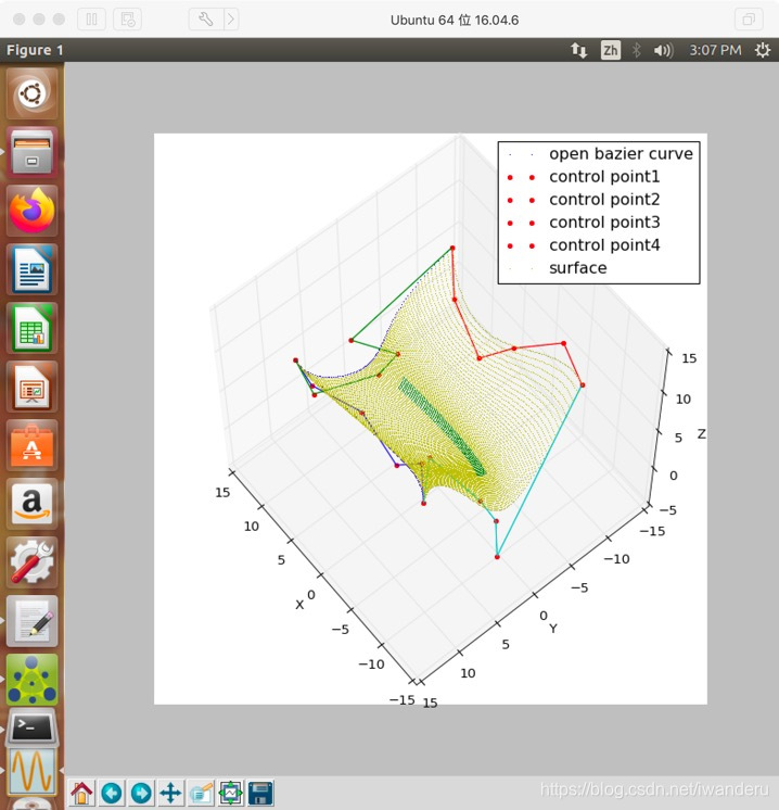
第五步，绘制曲线

#5.show the boundary
plt.plot(f[:,0],f[:,1],f[:,2],'b.',markersize=1,label='open bazier curve')
plt.plot(point_curve1[:,0],point_curve1[:,1],point_curve1[:,2],'r.',markersize=8, label='control point1')
plt.plot(point_curve2[:,0],point_curve2[:,1],point_curve2[:,2],'r.',markersize=8, label='control point2')
plt.plot(point_curve3[:,0],point_curve3[:,1],point_curve3[:,2],'r.',markersize=8, label='control point3')
plt.plot(point_curve4[:,0],point_curve4[:,1],point_curve4[:,2],'r.',markersize=8, label='control point4')
plt.plot(point_curve1[:,0],point_curve1[:,1],point_curve1[:,2],'-',markersize=1)
plt.plot(point_curve2[:,0],point_curve2[:,1],point_curve2[:,2],'-',markersize=1)
plt.plot(point_curve3[:,0],point_curve3[:,1],point_curve3[:,2],'-',markersize=1)
plt.plot(point_curve4[:,0],point_curve4[:,1],point_curve4[:,2],'-',markersize=1)

#6.show the surface
surface_item = np.array([],dtype=np.float64)
Q00 = point_curve3[0]
Q01 = point_curve3[-1]
Q10 = point_curve1[0]
Q11 = point_curve1[-1]
for u in range(N):
  for v in range(N):
    surface_item = alpha_u[u]*f[4*v+3]+(1-alpha_u[u])*f[4*v+1] + beta_v[v]*f[4*u+2]+(1-beta_v[v])*f[4*u] - (beta_v[v]*(alpha_u[u]*Q00+(1-alpha_u[u])*Q01)+(1-beta_v[v])*(alpha_u[u]*Q10+(1-alpha_u[u])*Q11))
    #surface_item = u*f[4*v]+(1-u)*f[4*v+2] + v*f[4*v+1]+(1-v)*f[4*v+3] - (v*(u*Q00+(1-u)*Q01)+(1-v)*(u*f[4*v+1]+(1-u)*Q11))
    #plt.plot(surface_item[0],surface_item[1],surface_item[2],'y.',markersize=1)
    surface = np.append(surface,surface_item)

当然，如果也想显示出用户根据u，v的值选定的部分曲面的话，可以通过以下函数实现。

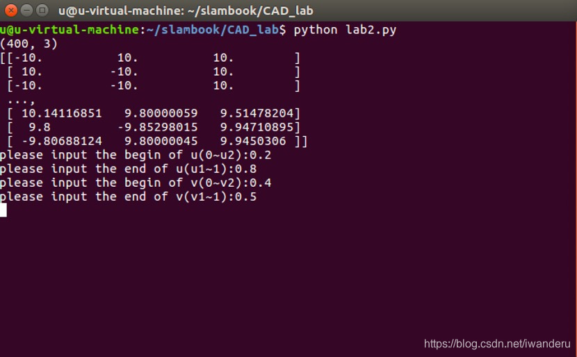
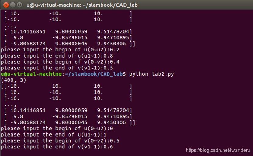
#7.show the selected part of the coon face
u1 = input("please input the begin of u(0~u2):") * N
u2 = input("please input the end of u(u1~1):") * N
v1 = input("please input the begin of v(0~v2):") * N
v2 = input("please input the end of v(v1~1):") * N
surface_selected = np.array([],dtype=np.float64)
for u in range(N):
  for v in range(N):
    if (u>=u1 and u<=u2 and v>=v1 and v<=v2):
      surface_item = alpha_u[u]*f[4*v+3]+(1-alpha_u[u])*f[4*v+1] + beta_v[v]*f[4*u+2]+(1-beta_v[v])*f[4*u] - (beta_v[v]*(alpha_u[u]*Q00+(1-alpha_u[u])*Q01)+(1-beta_v[v])*(alpha_u[u]*Q10+(1-alpha_u[u])*Q11))
      surface_selected = np.append(surface_selected,surface_item)

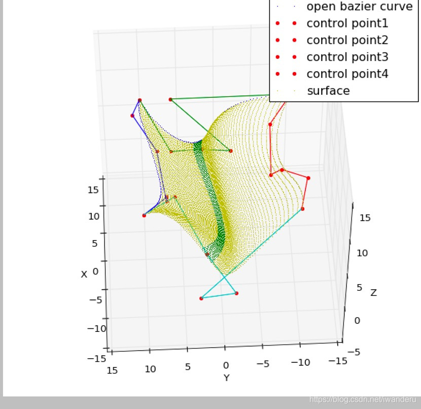
最后，注意数据格式是可以被pyplot所接受的。把plt.plot(surface[:,0],surface[:,1],surface[:,2],‘y.’,markersize=1, label=‘surface’)中的’y.‘改为’-'可以显示连续的曲面。

surface = surface.reshape((-1,3))
surface_selected = surface_selected.reshape((-1,3))
plt.plot(surface[:,0],surface[:,1],surface[:,2],'y.',markersize=1, label='surface')
plt.plot(surface_selected[:,0],surface_selected[:,1],surface_selected[:,2],'g.',markersize=1)

ax.legend()
ax.set_xlabel('X')
ax.set_ylabel('Y')
ax.set_zlabel('Z')
plt.show()