MATLAB实例:散点密度图
作者:凯鲁嘎吉 - 博客园 http://www.cnblogs.com/kailugaji/
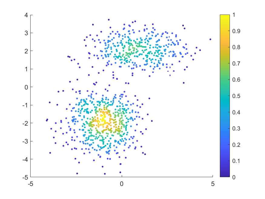
MATLAB绘制用颜色表示数据密度的散点图
数据来源:MATLAB中“fitgmdist”的用法及其GMM聚类算法,将数据保存为gauss.txt
1. demo.m
% 用颜色表示数据密度的散点图
data_load=dlmread('E:\scanplot\gauss.txt');
X=data_load(:,1:2);
scatplot(X(:,1),X(:,2),'circles', sqrt((range(X(:, 1))/30)^2 + (range(X(:,2))/30)^2), 100, 5, 1, 8);
print(gcf,'-dpng','散点密度图.png');
2. scatplot.m
来自:https://www.mathworks.com/matlabcentral/fileexchange/8577-scatplot
function out = scatplot(x,y,method,radius,N,n,po,ms)
% Scatter plot with color indicating data density
% https://www.mathworks.com/matlabcentral/fileexchange/8577-scatplot
% USAGE:
%   out = scatplot(x,y,method,radius,N,n,po,ms)
%   out = scatplot(x,y,dd)
%
% DESCRIPTION:
%   Draws a scatter plot with a colorscale
%   representing the data density computed
%   using three methods
%
% INPUT VARIABLES:
%   x,y - are the data points
%   method - is the method used to calculate data densities:
%       'circles' - uses circles with a determined area
%               centered at each data point
%       'squares' - uses squares with a determined area
%               centered at each data point
%       'voronoi' - uses voronoi cells to determin data densities
%               default method is 'voronoi'
%   radius - is the radius used for the circles or squares
%       used to calculate the data densities if
%       (Note: only used in methods 'circles' and 'squares'
%           default radius is sqrt((range(x)/30)^2 + (range(y)/30)^2)
%   N - is the size of the square mesh (N x N) used to
%       filter and calculate contours
%       default is 100
%   n - is the number of coeficients used in the 2-D
%       running mean filter
%       default is 5
%       (Note: if n is length(2), n(2) is tjhe number of
%       of times the filter is applied)
%   po - plot options:
%       0 - No plot
%       1 - plots only colored data points (filtered)
%       2 - plots colored data points and contours (filtered)
%       3 - plots only colored data points (unfiltered)
%       4 - plots colored data points and contours (unfiltered)
%           default is 1
%   ms - uses this marker size for filled circles
%       default is 4
%
% OUTPUT VARIABLE:
%   out - structure array that contains the following fields:
%       dd - unfiltered data densities at (x,y)
%       ddf - filtered data densities at (x,y)
%       radius - area used in 'circles' and 'squares'
%               methods to calculate densities
%       xi - x coordenates for zi matrix
%       yi - y coordenates for zi matrix
%       zi - unfiltered data densities at (xi,yi)
%       zif - filtered data densities at (xi,yi)
%       [c,h] = contour matrix C as described in
%           CONTOURC and a handle H to a contourgroup object
%       hs = scatter points handles
%
%Copy-Left, Alejandro Sanchez-Barba, 2005

if nargin==0
    scatplotdemo
    return
end
if nargin<3 | isempty(method)
    method = 'vo';
end
if isnumeric(method)
   gsp(x,y,method,2)
   return
else
    method = method(1:2);
end
if nargin<4 | isempty(n)
    n = 5; %number of filter coefficients
end
if nargin<5 | isempty(radius)
    radius = sqrt((range(x)/30)^2 + (range(y)/30)^2);
end
if nargin<6 | isempty(po)
    po = 1; %plot option
end
if nargin<7 | isempty(ms)
    ms = 7; %markersize
end
if nargin<8 | isempty(N)
    N = 100; %length of grid
end
%Correct data if necessary
x = x(:);
y = y(:);
%Asuming x and y match
idat = isfinite(x);
x = x(idat);
y = y(idat);
holdstate = ishold;
if holdstate==0
    cla
end
hold on
%--------- Caclulate data density ---------
dd = datadensity(x,y,method,radius);
%------------- Gridding -------------------
xi = repmat(linspace(min(x),max(x),N),N,1);
yi = repmat(linspace(min(y),max(y),N)',1,N);
zi = griddata(x,y,dd,xi,yi);
%----- Bidimensional running mean filter -----
zi(isnan(zi)) = 0;
coef = ones(n(1),1)/n(1);
zif = conv2(coef,coef,zi,'same');
if length(n)>1
    for k=1:n(2)
        zif = conv2(coef,coef,zif,'same');
    end
end
%-------- New Filtered data densities --------
ddf = griddata(xi,yi,zif,x,y);
%----------- Plotting --------------------
switch po
    case {1,2}
        if po==2
            [c,h] = contour(xi,yi,zif);
            out.c = c;
            out.h = h;
        end %if
        hs = gsp(x,y,ddf,ms);
        out.hs = hs;
        colorbar
    case {3,4}
        if po>3
            [c,h] = contour(xi,yi,zi);
            out.c = c;
        end %if
        hs = gsp(x,y,dd,ms);
        out.hs = hs;
        colorbar
end %switch
%------Relocate variables and place NaN's ----------
dd(idat) = dd;
dd(~idat) = NaN;
ddf(idat) = ddf;
ddf(~idat) = NaN;
%--------- Collect variables ----------------
out.dd = dd;
out.ddf = ddf;
out.radius = radius;
out.xi = xi;
out.yi = yi;
out.zi = zi;
out.zif = zif;
if ~holdstate
    hold off
end
return
%~~~~~~~~~~~~~~~~~~~~~~~~~~~~~~~~~~~~~~
function scatplotdemo
po = 2;
method = 'squares';
radius = [];
N = [];
n = [];
ms = 5;
x = randn(1000,1);
y = randn(1000,1);

out = scatplot(x,y,method,radius,N,n,po,ms)

return
%~~~~~~~~~~ Data Density ~~~~~~~~~~~~~~
function dd = datadensity(x,y,method,r)
%Computes the data density (points/area) of scattered points
%Striped Down version
%
% USAGE:
%   dd = datadensity(x,y,method,radius)
%
% INPUT:
%   (x,y) -  coordinates of points
%   method - either 'squares','circles', or 'voronoi'
%       default = 'voronoi'
%   radius - Equal to the circle radius or half the square width
Ld = length(x);
dd = zeros(Ld,1);
switch method %Calculate Data Density
    case 'sq'  %---- Using squares ----
        for k=1:Ld
            dd(k) = sum( x>(x(k)-r) & x<(x(k)+r) & y>(y(k)-r) & y<(y(k)+r) );
        end %for
        area = (2*r)^2;
        dd = dd/area;
    case 'ci'
        for k=1:Ld
            dd(k) = sum( sqrt((x-x(k)).^2 + (y-y(k)).^2) < r );
        end
        area = pi*r^2;
        dd = dd/area;
    case 'vo'  %----- Using voronoi cells ------
        [v,c] = voronoin([x,y]);
        for k=1:length(c)
            %If at least one of the indices is 1,
            %then it is an open region, its area
            %is infinity and the data density is 0
            if all(c{k}>1)
                a = polyarea(v(c{k},1),v(c{k},2));
                dd(k) = 1/a;
            end %if
        end %for
end %switch
return
%~~~~~~~~~~ Graf Scatter Plot ~~~~~~~~~~~
function varargout = gsp(x,y,c,ms)
%Graphs scattered poits
map = colormap;
ind = fix((c-min(c))/(max(c)-min(c))*(size(map,1)-1))+1;
h = [];
%much more efficient than matlab's scatter plot
for k=1:size(map,1)
    if any(ind==k)
        h(end+1) = line('Xdata',x(ind==k),'Ydata',y(ind==k), ...
            'LineStyle','none','Color',map(k,:), ...
            'Marker','.','MarkerSize',ms);
    end
end
if nargout==1
    varargout{1} = h;
end
return
3. 结果