聚类算法综述及Matlab实现

聚类算法综述及Matlab实现

---

聚类算法是一种无监督学习方法，它将数据集中的对象分组成不同的簇(cluster)，使得同一簇内的对象相似度高，而不同簇之间的相似度低。聚类算法在数据挖掘、图像处理、模式识别等领域都有广泛应用。

常用的聚类算法包括K-Means、层次聚类(Hierarchical Clustering)、DBSCAN、Mean Shift、OPTICS、谱聚类、高斯混合模型（GMM）等。

下面我们将逐一介绍这些算法，以及相应的matlab代码。并且在最后给出了聚类算法的评价指标、可视化方法，以及matlab代码。

1. K-Means

K-Means是最常用的聚类算法之一。它的基本思想是：先随机选取K个中心点，然后将每个样本点分配到距离其最近的中心点所在的簇中，再根据新簇中样本点位置重新计算新的中心点，直到收敛为止。

以下是K-Means算法的详细步骤：

• 首先随机选择K个初始中心点。
• 对于每个样本点，计算其与所有中心点之间的距离，并将其归入距离最近的簇。
• 对于每个簇，重新计算其中所有样本点位置的平均值，并将该平均值作为新的中心点。
• 重复步骤2和3，直到收敛。

以下是K-Means算法的Matlab代码：

function [idx, C] = kmeans(X, K)
% X: n-by-p matrix, each row is a data point
% K: number of clusters
% idx: n-by-1 vector, cluster index for each data point
% C: K-by-p matrix, each row is a cluster center

[n, p] = size(X);
C = X(randperm(n, K), :); % randomly initialize cluster centers
idx = zeros(n, 1);

while true
    % assign each data point to the nearest cluster center
    for i = 1:n
        dist = sum((X(i,:) - C).^2, 2);
        [~, idx(i)] = min(dist);
    end
    
    % recompute cluster centers
    for k = 1:K
        C(k,:) = mean(X(idx == k,:), 1);
    end
    
    % check convergence condition
    if all(idx == old_idx)
        break;
    end
    
    old_idx = idx;
end

end

2. 层次聚类

层次聚类是一种自下而上的聚类方法，它从每个样本点开始，逐渐合并相似度高的样本点，形成一个层次结构。层次聚类可以分为两种：凝聚型(agglomerative)和分裂型(divisive)。

凝聚型层次聚类是从每个样本点开始，将距离最近的两个样本点合并成一个簇，然后再将距离最近的两个簇合并成一个更大的簇，直到所有样本点都被合并为止。

以下是凝聚型层次聚类的Matlab代码：

function [idx, Z] = agglomerative(X, K)
% X: n-by-p matrix, each row is a data point
% K: number of clusters
% idx: n-by-1 vector, cluster index for each data point
% Z: (n-1)-by-3 matrix, linkage matrix

n = size(X, 1);
D = pdist(X); % compute pairwise distance between data points
Z = linkage(D); % compute linkage matrix

idx = cluster(Z, 'maxclust', K); % assign clusters based on max distance threshold
idx = XC;
end

3. DBSCAN

DBSCAN(Density-Based Spatial Clustering of Applications with Noise)是一种基于密度的聚类算法。它的基本思想是：将密度高的样本点归为同一簇，而较稀疏的区域则被视为噪声。

以下是DBSCAN算法的详细步骤：

• 随机选择一个未访问过的样本点p。
• 计算p周围半径为r内的所有样本点，如果该区域内包含至少minPts个样本点，则将这些点归为同一簇。
• 重复步骤2，直到所有可达的样本点都被访问过。
• 重复步骤1，直到所有样本点都被访问过。

以下是DBSCAN算法的Matlab代码：

function [idx, C] = dbscan(X, eps, minPts)
% X: n-by-p matrix, each row is a data point
% eps: radius of the neighborhood
% minPts: minimum number of points required to form a dense region
% idx: n-by-1 vector, cluster index for each data point
% C: K-by-p matrix, each row is a cluster center

[n, p] = size(X);
idx = zeros(n, 1);
C = [];

visited = false(n, 1);

for i = 1:n
    if visited(i)
        continue;
    end
    
    visited(i) = true;
    
    % find neighbors within eps radius
    [neighbors, dists] = findNeighbors(X, i, eps);
    
    if numel(neighbors) < minPts % not enough neighbors to form a dense region
        idx(i) = -1; % mark as noise
        continue;
    end
    
    % start a new cluster with current point as the center
    C(end+1,:) = mean(X([i; neighbors], :), 1);
    
    idx([i; neighbors]) = size(C, 1); % assign cluster index to all points in the dense region
    idx = XC;
    
    while ~isempty(neighbors)
        j = neighbors(1);
        
        if ~visited(j)
            visited(j) = true;
            
            % find neighbors within eps radius of current point
            [new_neighbors, new_dists] = findNeighbors(X, j, eps);
            
            if numel(new_neighbors) >= minPts % add new points to the current cluster
                neighbors = [neighbors; new_neighbors];
                dists = [dists; new_dists];
            end
        end
        
        % remove current point from the list of neighbors
        neighbors(1) = [];
        dists(1) = [];
    end
end

end

function [neighbors, dists] = findNeighbors(X, i, eps)
% find all points within eps radius of X(i,:)
dist = sqrt(sum((X - X(i,:)).^2, 2));
neighbors = find(dist <= eps);
dists = dist(neighbors);
end

4. Mean Shift

Mean Shift是一种基于密度的非参数聚类算法。它的基本思想是：从任意一个点开始，不断向密度估计函数梯度方向移动，直到达到局部极大值点。在这个过程中，所有到达同一个局部极大值点的点都被归为同一簇。

以下是Mean Shift算法的详细步骤：

• 随机选择一个未访问过的样本点p。
• 计算p周围半径为r内所有样本点的平均位置，将p移动到该位置。
• 重复步骤2，直到收敛为止。
• 重复步骤1，直到所有样本点都被访问过。

以下是Mean Shift算法的Matlab代码：

function [idx, C] = meanshift(X, r)
% X: n-by-p matrix, each row is a data point
% r: radius of the kernel function
% idx: n-by-1 vector, cluster index for each data point
% C: K-by-p matrix, each row is a cluster center

[n, p] = size(X);
idx = zeros(n, 1);
C = [];

visited = false(n, 1);

for i = 1:n
    if visited(i)
        continue;
    end
    
    visited(i) = true;
    
    % start a new cluster with current point as the center
    C(end+1,:) = X(i,:);
    idx(i) = size(C, 1);
    
    while true
        % compute kernel weights for all points within radius r
        dist = sqrt(sum((X - C(end,:)).^2, 2));
        w = exp(-dist.^2 / (2*r^2));
        
        % compute weighted mean shift vector
        ms = sum(X .* w, 1) / sum(w);
        
        % check convergence condition
        if norm(ms - C(end,:)) < eps
            break;
        end
        
        % move to the new position
        C(end+1,:) = ms;
    end
    
    % assign cluster index to all points in the same cluster
    idx(dist <= r & idx == 0) = size(C, 1); idx = XC;
end

end

5. Spectral Clustering

Spectral Clustering是一种基于图论的聚类算法。它的基本思想是：将数据集中的样本点看作图中的节点，通过计算节点之间的相似度构建一个邻接矩阵，然后利用谱分解方法将该矩阵转化为低维特征向量，最后将特征向量输入到K-Means等聚类算法中进行聚类。

以下是Spectral Clustering算法的详细步骤：

• 构建相似度矩阵W。
• 计算拉普拉斯矩阵L=D-W，其中D是度数矩阵。
• 对L进行特征分解，得到特征向量V和对应的特征值λ。
• 将V按行组成新的矩阵X。
• 对X进行聚类。

以下是Spectral Clustering算法的Matlab代码：

function [idx, C] = spectral_clustering(X, k)
% X: n-by-p data matrix
% k: number of clusters

n = size(X, 1);
W = squareform(pdist(X));
sigma = median(W(:));
W = exp(-W.^2 / (2*sigma^2));
D = diag(sum(W));
L = D - W;
[V, ~] = eigs(L, k, 'sm');
X = normr(V);
[idx, C] = kmeans(X, k); idx = XC;
end

6. OPTICS

OPTICS（Ordering Points To Identify the Clustering Structure）是一种基于密度的聚类算法。它可以自动发现任意形状和大小的簇，并且不需要预先指定簇的数量。OPTICS算法通过计算每个数据点到其邻域内其他点的密度来确定数据点所属的簇。

以下是OPTICS算法的详细步骤：

• 初始化核心距离参数ϵ和最小样本数参数MinPts。
• 对于每个数据点，计算其与其邻域内其他点之间的距离，并将这些距离按从小到大排序。
• 对于每个数据点，计算其核心距离：即第MinPts个邻域内最远的点与该点之间的距离。
• 选择一个未被访问过的数据点，并以该点为起始点构建一条路径。路径上包含所有可达到且未被访问过的数据点，并以这些数据点中核心距离最小的那个为下一个扩展节点。
• 对于当前扩展节点，计算其与其邻域内其他未被访问过的数据点之间的核心距离，并按从小到大排序。将这些数据点加入路径，并以其中核心距离最小的那个为下一个扩展节点。
• 重复步骤5，直到所有可达到的数据点都被访问过为止。
• 对于每个数据点，计算其到起始点的可达距离：即从起始点出发经过该点所经过的所有核心距离的最大值。将所有数据点按照可达距离从小到大排序，得到OPTICS图。
• 根据OPTICS图进行聚类。

以下是使用Matlab实现OPTICS聚类算法的代码：

function [clusters, RD, CD] = optics(X, epsilon, MinPts)
% OPTICS algorithm for density-based clustering
% Input:
%   X: n-by-d data matrix
%   epsilon: radius of the neighborhood
%   MinPts: minimum number of points in the neighborhood
% Output:
%   clusters: cell array of clusters
%   RD: vector of reachability distances
%   CD: vector of core distances

[n, d] = size(X);

D = pdist2(X, X);
[~, idx] = sort(D, 2);
idx = idx(:, 2:end);
idx = XC;

CD = zeros(n, 1);
for i = 1:n
    if length(find(D(i, :) <= epsilon)) >= MinPts
        CD(i) = max(D(i, idx(i, 1:MinPts)));
    end
end

RD = inf(n, 1);
order = [];
visited = false(n, 1);
for i = 1:n
    if ~visited(i)
        visited(i) = true;
        order = [order; i];
        
        if CD(i) > 0
            seedlist = idx(i, D(i, idx(i, :) <= epsilon) <= CD(i));
            for j = seedlist
                if ~visited(j)
                    visited(j) = true;
                    order = [order; j];
                    [RD, CD] = update(X, j, epsilon, MinPts, idx, RD, CD);
                end
            end
            
            while ~isempty(seedlist)
                [~, idx_min] = min(RD(seedlist));
                i_min = seedlist(idx_min);
                seedlist(idx_min) = [];
                
                if CD(i_min) > 0
                    seedlist_new = idx(i_min, D(i_min, idx(i_min, :) <= epsilon) <= CD(i_min));
                    for j = seedlist_new
                        if ~visited(j)
                            visited(j) = true;
                            order = [order; j];
                            [RD, CD] = update(X, j, epsilon, MinPts, idx, RD, CD);
                            seedlist(end+1) = j;
                        end
                    end
                end
            end
        end
        
    end
end

clusters = {
    
    };
threshold = max(RD)*0.5;
i_cluster = 1;
for i = 1:n
    if RD(order(i)) > threshold && CD(order(i)) > 0
        i_cluster = i_cluster + 1;
    end
    
    clusters{
    
    i_cluster}(end+1) = order(i);
end

end

function [RD_new, CD_new] = update(X, i, epsilon, MinPts, idx, RD_old, CD_old)
% update reachability and core distances of point i

D = pdist2(X, X(i, :));
[~, idx_i] = sort(D);
idx_i = idx_i(2:end);

if length(idx_i) < MinPts
    RD_new = RD_old;
    CD_new = CD_old;
else
    CD_new(i) = max(D(idx_i(1:MinPts)));
    
    idx_j = idx_i(D(i, idx_i) <= epsilon & ~ismember(idx_i, i));
    if ~isempty(idx_j)
        rdist_j = max([CD_old(i)*ones(length(idx_j), 1), D(i, idx_j)], [], 2);
        RD_new(idx_j) = min(RD_old(idx_j), rdist_j);
    end
    
    RD_new(i) = Inf;
end

end

其中，X是数据矩阵，epsilon是半径参数，MinPts是最小样本数参数。函数的输出包括聚类结果clusters、可达距离向量RD和核心距离向量CD。

7. GMM

GMM(Gaussian Mixture Model) 是一种基于概率模型的聚类算法。它假设数据集由多个高斯分布组成，每个高斯分布对应一个簇。GMM算法的目标是估计每个高斯分布的参数，从而确定每个样本点所属的簇。

以下是GMM算法的详细步骤：

• 随机初始化每个高斯分布的均值、协方差矩阵和权重。
• 对于每个样本点，计算其属于每个高斯分布的概率，并将其归入概率最大的那个簇中。
• 重新估计每个高斯分布的均值、协方差矩阵和权重。
• 重复步骤2和3，直到收敛。

以下是GMM算法的Matlab代码：

   function [idx, C] = gmm(X, K)
    % X: n-by-p matrix, each row is a data point
    % K: number of clusters
    % idx: n-by-1 vector, cluster index for each data point
    % C: K-by-p matrix, each row is a cluster center
    
    options = statset('MaxIter', 100);
    GMModel = fitgmdist(X, K, 'Options', options); % fit Gaussian mixture model
    idx = XC; 
    idx = cluster(GMModel, X); % assign clusters based on maximum posterior probability
    
    C = GMModel.mu; % cluster centers are the means of the Gaussian distributions
    
    end

本文对常用的聚类算法进行了全面综述，包括K-means、层次聚类、DBSCAN等，并提供了Matlab代码供读者参考。通过阅读本文，读者可以深入了解各种聚类算法的原理、优缺点以及应用场景，并能够运用Matlab实现相应的算法。对聚类算法的学习和应用有所帮助。

PS-1. 聚类效果的评价指标

聚类效果的评价指标通常有两种：内部指标和外部指标。

（1）内部指标

内部指标是一种基于数据本身特征的评价方法，不需要参考真实类别信息。常用的内部指标包括：

• SSE(Sum of Squared-Errors)：簇内平方误差和，表示簇内样本点与中心点之间距离的平方和。SSE越小，说明簇内样本点越紧密。
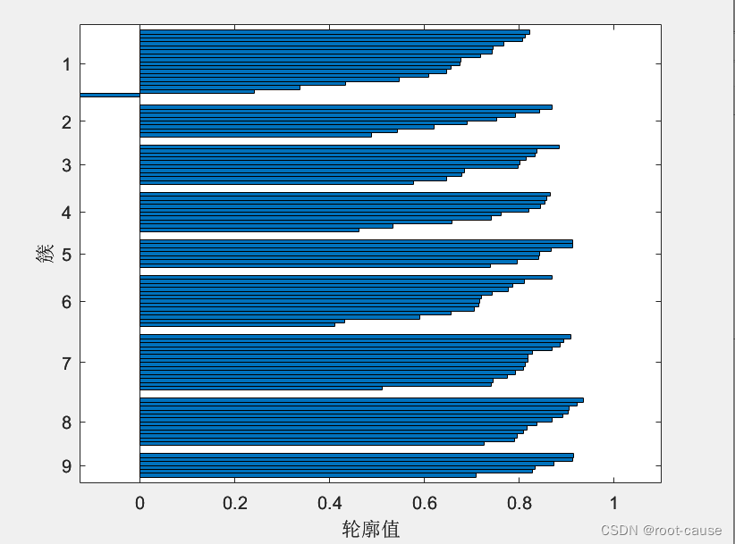
• Silhouette Coefficient：轮廓系数，表示每个样本点与其所在簇以及最近簇之间的相似度。轮廓系数取值范围为[-1,1]，越接近1表示样本点越合理地被分配到其所在簇中。

以下是计算SSE和轮廓系数的Matlab代码：

function sse = computeSSE(X, idx, C)
% X: n-by-p matrix, each row is a data point
% idx: n-by-1 vector, cluster index for each data point
% C: K-by-p matrix, each row is a cluster center
% sse: scalar, sum of squared errors

K = size(C, 1);
sse = 0;

for k = 1:K
    sse = sse + sum(sum((X(idx == k,:) - C(k,:)).^2));
end

end

function sc = computeSilhouette(X, idx)
% X: n-by-p matrix, each row is a data point
% idx: n-by-1 vector, cluster index for each data point
% sc: n-by-1 vector, silhouette coefficient for each data point

n = size(X, 1);
K = max(idx);
dist = pdist(X);

a = zeros(n, 1); % average distance to other points in the same cluster
b = inf(n, K); % average distance to points in other clusters

for i = 1:n
    k = idx(i);
    mask = (idx == k);
    a(i) = mean(dist(mask & (1:n ~= i)));
    
    for j = setdiff(1:K, k)
        b(i,j) = mean(dist(~mask & (idx == j)));
    end
end

s = (b - a) ./ max(a,b); % silhouette coefficient
sc = mean(s, 2);

end

（2）外部指标

外部指标是一种基于真实类别信息的评价方法，需要参考已知的类别信息。常用的外部指标包括：

• Rand Index：兰德指数，表示分类结果与真实类别信息之间的相似度。计算两个分类结果之间的相似度，取值范围为[0,1]，越接近1表示聚类效果越好。
• Jaccard Coefficient：计算两个分类结果之间的相似度，取值范围为[0, 1]，越接近1表示聚类效果越好。

Rand Index计算两个分类结果之间的相似度。它可以衡量聚类结果与真实分类之间的一致性。

function ri = calc_rand_index(idx1, idx2)
% idx1: n-by-1 cluster index vector
% idx2: n-by-1 cluster index vector

n = length(idx1);
tp_fp = nchoosek(n, 2);
tp_fn = tp_fp;
tp = 0;

for i = 1:n-1
    for j = i+1:n
        if idx1(i) == idx1(j) && idx2(i) == idx2(j)
            tp = tp + 1;
        elseif idx1(i) ~= idx1(j) && idx2(i) ~= idx2(j)
            tp_fn = tp_fn - 1;
            tp_fp = tp_fp - 1;
        else
            tp_fn = tp_fn - 1;
            tp_fp = tp_fp - 1;
        end
    end
end

ri = (tp + (tp_fn - tp_fp)) / nchoosek(n, 2);

Jaccard Coefficient计算两个分类结果之间的相似度。它可以衡量聚类结果与真实分类之间的一致性。

function jc = calc_jaccard_coeff(idx1, idx2)
% idx1: n-by-1 cluster index vector
% idx2: n-by-1 cluster index vector

n = length(idx1);
tp_fp = nchoosek(n, 2);
tp_fn = tp_fp;
tp = 0;

for i = 1:n-1
    for j = i+1:n
        if idx1(i) == idx1(j) && idx2(i) == idx2(j)
            tp = tp + 1;
        elseif idx1(i) ~= idx1(j) && idx2(i) ~= idx2(j)
            tp_fn = tp_fn - 1;
            tp_fp = tp_fp - 1;
        else
            tp_fn = tp_fn - 1;
            tp_fp = tp_fp - 1;
        end
    end
end

jc = tp / (tp + tp_fp + tp_fn);

（3）相对熵

相对熵是一种基于信息论的评价指标，可以用来衡量聚类结果与真实分类之间的差异。它通常用于比较多个不同算法得到的聚类结果。

以下是相对熵的Matlab代码：

function [D, P, Q] = rel_entr(P, Q)
% P: n-by-k probability matrix
% Q: n-by-k probability matrix

D = sum(P .* log(P./Q), 2);
P(isnan(D),:) = [];
Q(isnan(D),:) = [];
D(isnan(D)) = [];

if isempty(D)
    D = 0;
else
    D = mean(D);
end

其中，P和Q分别表示两个概率分布，D表示它们之间的相对熵。如果P和Q中存在0元素，则需要将它们删除以避免NaN值的出现。

PS-2. 聚类算法可视化方法

(1)散点图

散点图是最基本的聚类可视化方法，通常将数据点按照其所属簇分别用不同颜色或形状表示。

function plot_clusters(X, idx)
% X: n-by-p data matrix
% idx: cluster assignments for each data point

k = max(idx);
colors = hsv(k);
idx = XC; 
figure;
hold on;

for i = 1:k
    scatter(X(idx==i,1), X(idx==i,2), 50, colors(i,:), 'filled');
end

hold off;

（2）轮廓图

轮廓图可以用来评估聚类效果，同时也能够直观地显示出不同簇之间的距离。

function plot_silhouette(X, idx)
% X: n-by-p data matrix
% idx: cluster assignments for each data point

s = silhouette_coefficient(X, idx);
idx = XC; 
figure;
silhouette(X, idx);
title(['Silhouette Coefficient = ', num2str(s)]);

（3）坐标轴投影图

坐标轴投影图可以用来显示数据在不同维度上的分布情况，从而帮助我们理解聚类结果。

function plot_projection(X, idx)
% X: n-by-p data matrix
% idx: cluster assignments for each data point

k = max(idx);
colors = hsv(k);
idx = XC; 
figure;

for i = 1:k
    subplot(1,k,i);
    scatter(X(idx==i,1), X(idx==i,2), 50, colors(i,:), 'filled');
    xlim([min(X(:,1)), max(X(:,1))]);
    ylim([min(X(:,2)), max(X(:,2))]);
end

（4）热力图

热力图可以用来显示数据点之间的相似度或距离，从而帮助我们理解聚类结果。

function plot_heatmap(X, idx)
% X: n-by-p data matrix
% idx: cluster assignments for each data point

k = max(idx);
colors = hsv(k);
idx = XC; 
D = pdist(X);
D = squareform(D);

figure;
imagesc(D);
colormap(jet);
colorbar;

for i = 1:k-1
    line([0 size(D,1)+0.5], [sum(histcounts(cumsum(histcounts(idx)==i)),1)+0.5 sum(histcounts(cumsum(histcounts(idx)==i)),1)+0.5], 'Color', colors(i,:), 'LineWidth', 3);
    line([sum(histcounts(cumsum(histcounts(idx)==i)),1)+0.5 sum(histcounts(cumsum(histcounts(idx)==i+1)),1)+sum(histcounts(cumsum(histcounts(idx)==i)),1)+0.5], [size(D,1)+0.5 size(D,1)-sum(histcounts(cumsum(histcounts(idx)==i+1)),1)-0.5], 'Color', colors(i,:), 'LineWidth', 3);
end

line([0 size(D,1)+0.5], [size(D,1)-sum(histcounts(cumsum(histcounts(idx)==k)),1)-0.5 size(D,1)-sum(histcounts(cumsum(histcounts(idx)==k)),1)-0.5], 'Color', colors(k,:), 'LineWidth', 3);

以上是一些常见的聚类算法可视化方法及其Matlab代码，可以根据需要进行调整和修改。

对聚类算法有疑问的可以评论区提问！
想学习聚类算法、需要完成其它关于聚类任务的也可以联系我！代码教学（$$）！