模型的方差与偏差
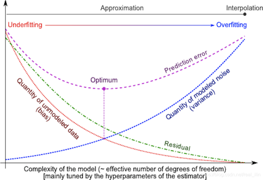
每种模型都有优点和缺点,一个模型的泛化误差可以分解为偏差(bias)、方差(variance)和噪音(noise)。偏差是不同训练集的平均误差,方差是对不同训练集的敏感程度,而噪音是数据本身的属性。为了使得方差和偏差最小(也就是泛化能力最大),常用的方法是选择算法(线性或非线性)及算法的超参数,另一种减小方差的方法是增加样本的数量,极限的情况是把所有的样本作为训练样本,那么就不存在方差的情况了。但是在实际的项目中,往往训练数量是无法增加的。
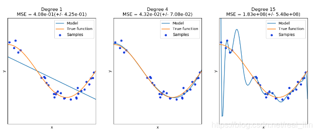
对于方程f(x)=cos(3* pi *x/2)的拟合,用了三个不同的多项式estimator,第一个是underfitting,模型太简单,偏差太大,第二个是nomal,正好拟合,第三个是overfitting,模型过于复杂,对不同的训练数据集非常敏感,也就是如果换了training set,模型的得分会特别差。
对于一维数据可以可视化,但是实际应用中,对于无法可视化的多维数据有两种方法可以使用:
- validation curve
- learning curve
Validation Curve
一个良好的模型是拥有好的泛化能力。为了评估模型,我们需要一个metric,也就是一个scoring function,比如accuracy,precision。选择多个超参数的方法有GridSearchCV或RandomiedSearchCV,但是在选择的超参数是基于validation set的上得分。如果我们是根据validation set上的得分来优化超参数,则验证分数会有偏差,就不再是对泛化能力的良好估计。理论上,为了得到对泛化能力的正确估计,必须在另一个测试集上计算得分。
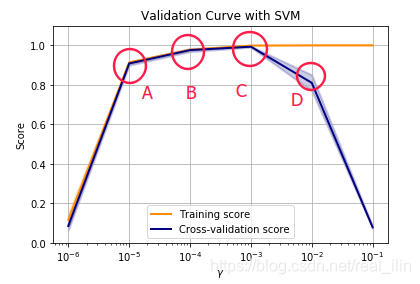
然而,有时候绘制单个超参数的training score和validation score可以判断模型的状态,是过拟合还欠拟合。
如下图,是使用SVC手写数字识别的多分类问题,横坐标代表超参数gamma的大小,y代表得分,分别有training score和cross-validation score。根据位置来判断:A、B代表欠拟合,C代表正好,D代表过拟合。
Learning Curve
学习曲线展示了随着样本数量的增加模型在验证集和训练集上的得分情况。从学习曲线中我们可以看出随着样本的增加模型的获益情况,以及模型处在什么样的状态。
随着样本的增加,validation score和training score都在一个比较低的水平,则此时为欠拟合,再增加样本也无法增加模型的score。使用Naive Bayes模型手写数字识别:
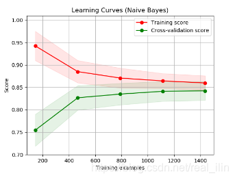
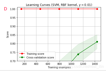
如果在最大样本数量的地方,training score比validation score大很多,则处理过过拟合的情况。下图中,training score一直处在比较高的位置,而validation score逐渐增大。虽然在training set上的score一起比较接近1,但是cross-validation score逐渐增大,最后两个点几乎重合,说明此时并没有过拟合。 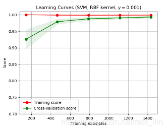
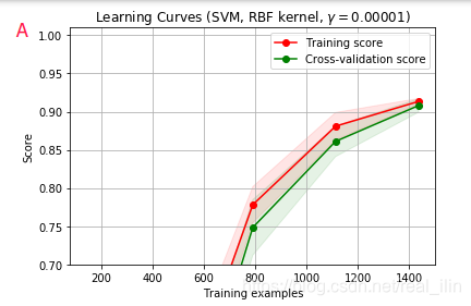
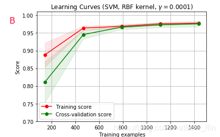
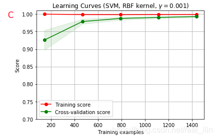
同样使用SVC,不同gamma的学习曲线对应validation curve中ABCD个点的情况,同样,AB为欠拟合,C为正好拟合,D为过拟合。A和D比较好区分,而B和C不好区分,B的training score在数据量小的情况,没并有达到接近1的位置,而C是。但两者的相同点是在数据量达到最达时两条线基本重合。如下:
代码:
%matplotlib inline
print(__doc__)

from sklearn.model_selection import validation_curve
param_range = np.array([1.0e-6,1.0e-5,1.0e-4,1.0e-3,1.0e-2,1.0e-1,])
train_scores, test_scores = validation_curve(
    SVC(), X, y, param_name="gamma", param_range=param_range,
    cv=cv, scoring="accuracy", n_jobs=1)
train_scores_mean = np.mean(train_scores, axis=1)
train_scores_std = np.std(train_scores, axis=1)
test_scores_mean = np.mean(test_scores, axis=1)
test_scores_std = np.std(test_scores, axis=1)

plt.title("Validation Curve with SVM")
plt.xlabel(r"$\gamma$")
plt.ylabel("Score")
plt.ylim(0.0, 1.1)
lw = 2
plt.semilogx(param_range, train_scores_mean, label="Training score",
             color="darkorange", lw=lw)
plt.fill_between(param_range, train_scores_mean - train_scores_std,
                 train_scores_mean + train_scores_std, alpha=0.2,
                 color="darkorange", lw=lw)
plt.semilogx(param_range, test_scores_mean, label="Cross-validation score",
             color="navy", lw=lw)
plt.fill_between(param_range, test_scores_mean - test_scores_std,
                 test_scores_mean + test_scores_std, alpha=0.2,
                 color="navy", lw=lw)
plt.legend(loc="best")
plt.grid()
plt.show()

import numpy as np
import matplotlib.pyplot as plt
from sklearn.naive_bayes import GaussianNB
from sklearn.svm import SVC
from sklearn.datasets import load_digits
from sklearn.model_selection import learning_curve
from sklearn.model_selection import ShuffleSplit


def plot_learning_curve(estimator, title, X, y, ylim=None, cv=None,
                        n_jobs=None, train_sizes=np.linspace(.1, 1.0, 5)):
    """
    Generate a simple plot of the test and training learning curve.

    Parameters
    ----------
    estimator : object type that implements the "fit" and "predict" methods
        An object of that type which is cloned for each validation.

    title : string
        Title for the chart.

    X : array-like, shape (n_samples, n_features)
        Training vector, where n_samples is the number of samples and
        n_features is the number of features.

    y : array-like, shape (n_samples) or (n_samples, n_features), optional
        Target relative to X for classification or regression;
        None for unsupervised learning.

    ylim : tuple, shape (ymin, ymax), optional
        Defines minimum and maximum yvalues plotted.

    cv : int, cross-validation generator or an iterable, optional
        Determines the cross-validation splitting strategy.
        Possible inputs for cv are:
          - None, to use the default 3-fold cross-validation,
          - integer, to specify the number of folds.
          - :term:`CV splitter`,
          - An iterable yielding (train, test) splits as arrays of indices.

        For integer/None inputs, if ``y`` is binary or multiclass,
        :class:`StratifiedKFold` used. If the estimator is not a classifier
        or if ``y`` is neither binary nor multiclass, :class:`KFold` is used.

        Refer :ref:`User Guide <cross_validation>` for the various
        cross-validators that can be used here.

    n_jobs : int or None, optional (default=None)
        Number of jobs to run in parallel.
        ``None`` means 1 unless in a :obj:`joblib.parallel_backend` context.
        ``-1`` means using all processors. See :term:`Glossary <n_jobs>`
        for more details.

    train_sizes : array-like, shape (n_ticks,), dtype float or int
        Relative or absolute numbers of training examples that will be used to
        generate the learning curve. If the dtype is float, it is regarded as a
        fraction of the maximum size of the training set (that is determined
        by the selected validation method), i.e. it has to be within (0, 1].
        Otherwise it is interpreted as absolute sizes of the training sets.
        Note that for classification the number of samples usually have to
        be big enough to contain at least one sample from each class.
        (default: np.linspace(0.1, 1.0, 5))
    """
    plt.figure()
    plt.title(title)
    if ylim is not None:
        plt.ylim(*ylim)
    plt.xlabel("Training examples")
    plt.ylabel("Score")
    train_sizes, train_scores, test_scores = learning_curve(
        estimator, X, y, cv=cv, n_jobs=n_jobs, train_sizes=train_sizes)
    train_scores_mean = np.mean(train_scores, axis=1)
    train_scores_std = np.std(train_scores, axis=1)
    test_scores_mean = np.mean(test_scores, axis=1)
    test_scores_std = np.std(test_scores, axis=1)
    plt.grid()

    plt.fill_between(train_sizes, train_scores_mean - train_scores_std,
                     train_scores_mean + train_scores_std, alpha=0.1,
                     color="r")
    plt.fill_between(train_sizes, test_scores_mean - test_scores_std,
                     test_scores_mean + test_scores_std, alpha=0.1, color="g")
    plt.plot(train_sizes, train_scores_mean, 'o-', color="r",
             label="Training score")
    plt.plot(train_sizes, test_scores_mean, 'o-', color="g",
             label="Cross-validation score")

    plt.legend(loc="best")
    return plt


digits = load_digits()
X, y = digits.data, digits.target


title = "Learning Curves (Naive Bayes)"
# Cross validation with 100 iterations to get smoother mean test and train
# score curves, each time with 20% data randomly selected as a validation set.
cv = ShuffleSplit(n_splits=100, test_size=0.2, random_state=0)

estimator = GaussianNB()
plot_learning_curve(estimator, title, X, y, ylim=(0.7, 1.01), cv=cv, n_jobs=4)

plt.show()

ylim_min=0.7

title = r"Learning Curves (SVM, RBF kernel, $\gamma=0.00001$)"
plot_learning_curve(SVC(gamma=1.0e-5),title,X,y,(ylim_min,1.01),cv=cv,n_jobs=4)

title = r"Learning Curves (SVM, RBF kernel, $\gamma=0.0001$)"
# SVC is more expensive so we do a lower number of CV iterations:
cv = ShuffleSplit(n_splits=10, test_size=0.2, random_state=0)
estimator = SVC(gamma=1.0e-4)
plot_learning_curve(estimator, title, X, y, (ylim_min, 1.01), cv=cv, n_jobs=4)

title = r"Learning Curves (SVM, RBF kernel, $\gamma=0.0005$)"
plot_learning_curve(SVC(gamma=0.5e-3),title,X,y,(ylim_min,1.01),cv=cv,n_jobs=4)

title = r"Learning Curves (SVM, RBF kernel, $\gamma=0.001$)"
plot_learning_curve(SVC(gamma=1.0e-3),title,X,y,(ylim_min,1.01),cv=cv,n_jobs=4)

title = r"Learning Curves (SVM, RBF kernel, $\gamma=0.0015$)"
plot_learning_curve(SVC(gamma=1.5e-3),title,X,y,(ylim_min,1.01),cv=cv,n_jobs=4)

title = r"Learning Curves (SVM, RBF kernel, $\gamma=0.008$)"
plot_learning_curve(SVC(gamma=8e-3),title,X,y,(ylim_min,1.01),cv=cv,n_jobs=4)

title = r"Learning Curves (SVM, RBF kernel, $\gamma=0.01$)"
plot_learning_curve(SVC(gamma=1.0e-2),title,X,y,(ylim_min,1.01),cv=cv,n_jobs=4)

plt.show()
参考:https://scikit-learn.org/stable/modules/learning_curve.html