读书笔记-opencv-对比度增强-线性变换
灰度直方图
灰度直方图是图像的灰度函数,用来描述每个灰度级在图像矩阵中的像素数或者占有率。
python和C++实现
python实现:
import cv2
import  sys
import numpy as np
import matplotlib.pyplot as plt

def calcGrayHist(image):
	#灰度直方图的高宽
	rows, cols = image.shape[:2]
	#存储灰度直方图
	grayHist = np.zeros([256], np.uint64)
	for r in range(rows):
		for c in range(cols):
			grayHist[image[r][c]] += 1
	return grayHist

if __name__ == "__main__":
	imagePath = "G:/blog/OpenCV_picture/chapter4/img1.jpg"
	image = cv2.imread(imagePath, 0)
	try:
		image.shape
	except:
		print("fail read image!")

	#计算灰度直方图
	grayHist = calcGrayHist(image)

	#画出灰度直方图
	x_range = range(256)
	plt.plot(x_range, grayHist, 'r', linewidth = 2, c = 'black')
	#设置坐标轴的范围
	y_maxValue = np.max(grayHist)
	plt.axis([0,255, 0, y_maxValue])
	#设置坐标轴标签
	plt.xlabel('gray level')
	plt.ylabel("number of pixels")
	#显示灰度直方图
	plt.show()

	#Matplotlib 本身提供计算直方图的方法hist

	#将二维矩阵变成一维
	rows, cols = image.shape[:2]
	pixelSequence = image.reshape([rows * cols])

	#组数
	numberBins = 256

	#计算灰度直方图
	histoGray, bins, patch = plt.hist(pixelSequence, numberBins, facecolor = 'black', histtype= 'bar')
	#设置坐标轴的范围
	y_maxValue = np.max(grayHist)
	plt.axis([0,255, 0, y_maxValue])
	#设置坐标轴标签
	plt.xlabel('gray level')
	plt.ylabel("number of pixels")
	#显示灰度直方图
	plt.show()
C++实现的代码块
Mat calGrayHist(const Mat & image)
{
	//存储256个灰度级的像素个数
    Mat histogray = Mat::zeros(Size(256, 1), CV_32SC1);

    //图像的宽和高
    int rows = image.rows;
    int cols = image.cols;

    //计算每个灰度级的个数
    for(int i=0; i<image.rows; i++)
    {
		for(int j=0; j<image.cols; j++)
        {
			int index = int(image.at<uchar>(i, j));
            histogray.at<int>(0, index) += 1;
        }
    }

    return histogray;
}
输出图片:
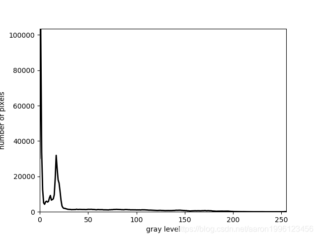
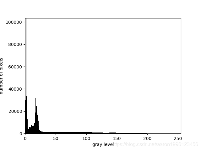
图像的对比度可以通过灰度级范围来度量的,而灰度级的范围可以通过观察灰度直方图得到,灰度级的范围越大代表的对比度越强。
线性变换
原理详解
假设输入的图像为I,宽为W,高为H,输出图像记为O,图像的线性变换可以表示为:
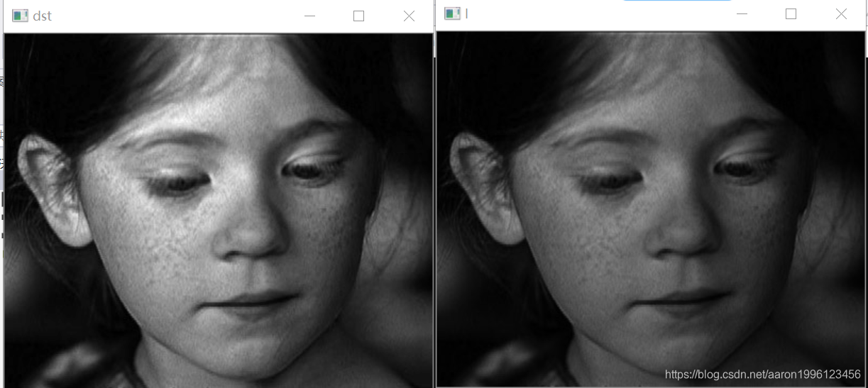
当a=1,b=0时,输出图像为原图像的一个副本,当a>1时,输出图像比原图像I的对比度有所增强,当0<a<1时,对比度减小。b对应的是输出图像的亮度,当b>0,亮度增强;当b<0亮度减弱。
对于图像矩阵的线性变换,通过点乘实现,有时需要注意数据类型的改变。对于一个8位图的对比增强,线性输出若大于255 需要将其截断为255,而不是取模运算。
python实现:
import sys
import cv2
import numpy as np
if __name__ == "__main__":
imagePath = "G:\\blog\\OpenCV_picture\\chapter4\\img4.jpg"
I = cv2.imread(imagePath, 0)
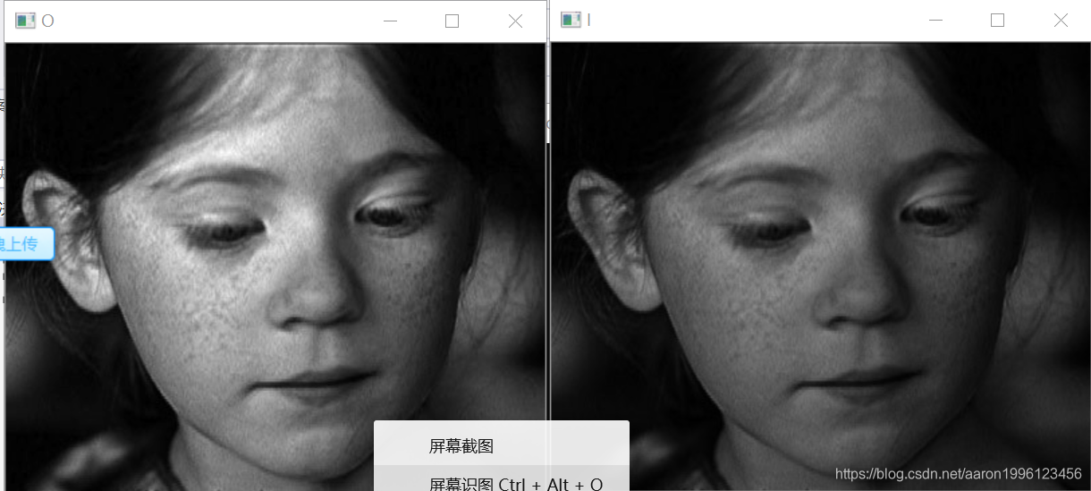
#线性变换
a = 2
O = float(2)*I
#进行数据截断,大于255赋值为255
O[O>255] = 255
#类型转换
O = np.round(O)
O = O.astype(np.uint8)
#显示原图和线性变换的结果
cv2.imshow("I", I)
cv2.imshow("O", O)
cv2.waitKey(0)
cv2.destroyAllWindows()


C++实现
//method one
//Mat::convertTo(OutputArray m, int rtype, double alpha = 1, double beta = 0);

Mat I = (Mat_<uchar>(2,2) << 0, 200, 23, 4);
Mat O;

I.convertTo(O, CV_8UC1, 2.0, 0);
//method two
Mat O =3.5 * I;
//method three
//convertScaleAbs(InputArray src, OutArray dst, double alpha =1, double beta = 0);
convertScaleAbs(I, O, 2.0, 0)
也可以分段线性变换,就是阈值在某一范围采用一种线性变换, 在另一范围采取又一种线性判断,类似于分段函数。
直方图正规化
原理详解
假设输入图像为I,高为H,宽慰W, I(r,c)代表I的第r行第c列的灰度值,将I中出现最小的灰度值记为Imin, 最大灰度几位Imax,即I(r,c)∈[Imin, Imax],为使输出图像O的灰度范围为[Omin, Omax], I(r, c)和O(r,c)做一下映射关系:
其中0<=r<H, 0<=c<w, O(r,c)代表Odell第r行第c列的灰度值,这个过程就是直方图正规化
python实现
	imagePath = "G:\\blog\\OpenCV_picture\\chapter4\\img4.jpg"
	I = cv2.imread(imagePath, 0)

	#原图像灰度值的最大值最小值
	Imax = np.max(I)
	Imin = np.min(I)
	#输出图像的最大最小值
	Omin, Omax = 0, 255
	#计算a, b的值
	a = float(Omax- Omin)/(Imax-Imin)
	b = Omin - a * Imin

	O = a*I + b
	#数据类型转换
	O = O.astype(np.uint8)


	#类型转换
	O = np.round(O)
	O = O.astype(np.uint8)

	#显示原图和线性变换的结果
	cv2.imshow("I", I)
	cv2.imshow("O", O)
	cv2.waitKey(0)
	cv2.destroyAllWindows()
C++实现
void minMaxLoc(InputArray src, double* minVal, double*maxVal=0, Point* minLoc=0, Point* maxLoc=0, InputArray mask= noArray())
C++ 提供可以得到最小最大值的函数,以及它们所在的位置,若不想得到赋值为NULL。
正规化函数normalize
opencv提供函数
void normalize(InputArray src, OutputArray dst, double alpha=1, double beta=0, int norm_type=NORM_L2, int dtype=-1, InputArray mask=noArray())
src 输入矩阵,dst结构元(类似于输出矩阵), alpha结构元的瞄点(和前文的a作用类似)beta浮士德操作次数(和前文的b作用类似),norm_type边界扩充类型,dtype边界扩充值。
矩阵范数:
(1)1-范数–计算矩阵中的绝对值的和:
(2) 2-范数–计算矩阵中值得平方喝的开方:
(3) 3 -范数–计算矩阵中的值得绝对值的最大值:
输入矩阵:
KaTeX parse error: Undefined control sequence: \matrix at position 13: a = \left[ \̲m̲a̲t̲r̲i̲x̲{ -55 & 80 \\ 1…
norm_type = NORM_L1时,计算src的1-范数:
dst的计算过程:
KaTeX parse error: Undefined control sequence: \matrix at position 49: …}+beta= \left[ \̲m̲a̲t̲r̲i̲x̲{ \frac{-55}{49…
norm_type = NORM_L2时,计算src的2-范数:
dst的计算过程:
KaTeX parse error: Undefined control sequence: \matrix at position 48: …2}+beta= \left[\̲m̲a̲t̲r̲i̲x̲{\frac{-55}{290…
norm_type = NORM_INF时,计算src的3-范数:
dst的计算过程:
KaTeX parse error: Undefined control sequence: \matrix at position 53: …y}+beta= \left[\̲m̲a̲t̲r̲i̲x̲{\frac{-55}{255…
norm_type = NORM_MINMAX时,计算src的4-范数:首先计算最小值,在计算最大值。
dst的计算过程:
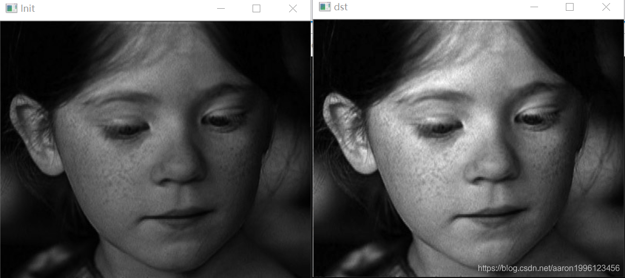
这个函数和前面的原理详解的方法一致。
python 实现
dst = cv2.normalize(I,None,255, 0, cv2.NORM_MINMAX, cv2.CV_8U)
C++实现
#include<opencv2/core.hpp>
#include<opencv2/imgproc.hpp>
#include<opencv2/highgui.hpp>
#include<iostream>

using namespace cv;

int main()
{

	//输入图像
	std::string imagePath = "G:\\blog\\OpenCV_picture\\chapter4\\img4.jpg";
	Mat src = imread(imagePath, 0);
	if (!src.data)
	{
		std::cout << "load image error!" << std::endl;
		return -1;
	}

	Mat dst;

	normalize(src, dst, 255, 0, NORM_MINMAX, CV_8U);

	imshow("Init", src);
	imshow("dst", dst);
	waitKey(0);
	return 0;
}