文章目录
- 1 Plotting Vectors
- 1.1 2D
- 1.2 3D
- 1.4 Euclidian Norm
- 1.5 Add
- 1.6 Geometric Translation
- 1.7 Multiplication by a Scalar
- 1.8 Normalized Vectors
- 1.9 Calculating the Angle between Vectors
- 1.10 Projecting a point onto an axis
- 2 Matrix
- 2.1 Diagonal matrix and Identity matrix
- 2.2 Matrix Multiplication
- 2.3 Matrix Transpose
- 2.3 Symmetric Matrix
- 3 Plotting a Matrix
1 Plotting Vectors
1.1 2D
以 2D 为例,画点
%matplotlib inline
import matplotlib.pyplot as plt
import numpy as np

u = np.array([2, 5])
v = np.array([3, 1])

x_coords, y_coords = zip(u, v)

plt.scatter(x_coords, y_coords, color=["r","b"])
plt.axis([0, 9, 0, 6])

plt.grid()
plt.show()

画有箭头的形式
def plot_vector2d(vector2d, origin=[0, 0], **options):
    return plt.arrow(origin[0], origin[1],
                     vector2d[0], vector2d[1],
                     head_width=0.2, head_length=0.3,
                     length_includes_head=True,**options)

plot_vector2d(u, color="r")
plot_vector2d(v, color="b")
plt.axis([0, 9, 0, 6])
plt.grid()
plt.show()

1.2 3D
先画点
%matplotlib inline
import matplotlib.pyplot as plt
import numpy as np

a = np.array([1, 2, 8])
b = np.array([5, 6, 3])

from mpl_toolkits.mplot3d import Axes3D

subplot3d = plt.subplot(111, projection='3d')
x_coords, y_coords, z_coords = zip(a,b)
subplot3d.scatter(x_coords, y_coords, z_coords,color=['r','b'])
# 设置坐标轴的范围
subplot3d.set_xlim3d([0, 9])
subplot3d.set_ylim3d([0, 9])
subplot3d.set_zlim3d([0, 9])
# 设置坐标轴的 label
subplot3d.set_xlabel("x")
subplot3d.set_ylabel("y")
subplot3d.set_zlabel("z")

plt.show()

加个往水平面上垂直的投影,让我们更好的知道空间的点在哪里!
%matplotlib inline
import matplotlib.pyplot as plt
import numpy as np

a = np.array([1, 2, 8])
b = np.array([5, 6, 3])

from mpl_toolkits.mplot3d import Axes3D

def plot_vectors3d(ax, vectors3d, z0, **options):
    for v in vectors3d:
        x, y, z = v
        ax.plot([x,x], [y,y], [z0, z], color="gray", linestyle='dotted', marker=".")
    x_coords, y_coords, z_coords = zip(*vectors3d)
    ax.scatter(x_coords, y_coords, z_coords, **options)

subplot3d = plt.subplot(111, projection='3d')

subplot3d.set_xlim3d([0, 9])
subplot3d.set_ylim3d([0, 9])
subplot3d.set_zlim3d([0, 9])

plot_vectors3d(subplot3d, [a,b], 0, color=("r","b"))
plt.show()

1.4 Euclidian Norm
也就向量的二范数,公式如下:
写个函数封装一下:
u = np.array([2, 5])

def vector_norm(vector):
    squares = [element**2 for element in vector]
    return sum(squares)**0.5

print("||", u, "|| = %s"% vector_norm(u))
output
|| [2 5] || = 5.385164807134504
其实呢,numpy 有现成的函数调用!
import numpy.linalg as LA
import numpy as np

u = np.array([2, 5])
LA.norm(u)
output
5.3851648071345037
验证一下计算的对不对(以二范数画圆)!
%matplotlib inline
import numpy.linalg as LA
import matplotlib.pyplot as plt

radius = LA.norm(u)

plt.gca().add_artist(plt.Circle((0,0), radius, color="#DDDDDD"))
plot_vector2d(u, color="red")
plt.axis([0, 8.7, 0, 6])
plt.grid()
plt.show()
def plot_vector2d 见前面 1.1 小节

Looks about right!
1.5 Add
import numpy as np

u = np.array([2, 5])
v = np.array([3, 1])

print(" ", u)
print("+", v)
print("-"*10)
print(" ",u + v)
output
  [2 5]
+ [3 1]
----------
  [5 6]
看看矢量加法对应的几何图像
%matplotlib inline
import matplotlib.pyplot as plt

plot_vector2d(u, color="r")
plot_vector2d(v, color="b")
plot_vector2d(v, origin=u, color="b", linestyle="dotted")
plot_vector2d(u, origin=v, color="r", linestyle="dotted")
plot_vector2d(u+v, color="g")

plt.axis([0, 9, 0, 7])
plt.text(0.7, 3, "u", color="r", fontsize=18)
plt.text(4, 3, "u", color="r", fontsize=18)
plt.text(1.8, 0.2, "v", color="b", fontsize=18)
plt.text(3.1, 5.6, "v", color="b", fontsize=18)
plt.text(2.4, 2.5, "u+v", color="g", fontsize=18)
plt.grid()
plt.show()
def plot_vector2d 见前面 1.1 小节

矢量的加法满足交换律(commutative)和结合律( associative).
- commutative:
- associative:
1.6 Geometric Translation
每个点都加一个 vector,就可以实现 translation
%matplotlib inline
import matplotlib.pyplot as plt
import numpy as np
# 原来的三个点
t1 = np.array([2, 0.25])
t2 = np.array([2.5, 3.5])
t3 = np.array([1, 2])

x_coords, y_coords = zip(t1, t2, t3, t1)
plt.plot(x_coords, y_coords, "c--", x_coords, y_coords, "co") # 前面画线,后面画圆点

# 加了矢量
plot_vector2d(v, t1, color="r", linestyle=":")
plot_vector2d(v, t2, color="r", linestyle=":")
plot_vector2d(v, t3, color="r", linestyle=":")

# 加了矢量后的三个点
t1b = t1 + v
t2b = t2 + v
t3b = t3 + v

x_coords_b, y_coords_b = zip(t1b, t2b, t3b, t1b)
plt.plot(x_coords_b, y_coords_b, "b-",x_coords_b, y_coords_b, "bo")# 前面画线,后面画圆点

plt.text(4, 4.2, "v", color="r", fontsize=18)
plt.text(3, 2.3, "v", color="r", fontsize=18)
plt.text(3.5, 0.4, "v", color="r", fontsize=18)

plt.axis([0, 6, 0, 5])
plt.grid()
plt.show()
def plot_vector2d 见前面 1.1 小节

1.7 Multiplication by a Scalar
import numpy as np
u = np.array([2, 5])
print("1.5 *", u, "=", 1.5*u)
output
1.5 * [2 5] = [3. 7.5]
可视化一下
%matplotlib inline
import matplotlib.pyplot as plt
import numpy as np

t1 = np.array([2, 0.25])
t2 = np.array([2.5, 3.5])
t3 = np.array([1, 2])

# 原来的三角
x_coords, y_coords = zip(t1, t2, t3, t1)
plt.plot(x_coords, y_coords, "c--", x_coords, y_coords, "co")
# 原来的vector
plot_vector2d(t1, color="r")
plot_vector2d(t2, color="r")
plot_vector2d(t3, color="r")

k = 2.5
t1c = k * t1
t2c = k * t2
t3c = k * t3
# scale后的三角
x_coords_c, y_coords_c = zip(t1c, t2c, t3c, t1c)
plt.plot(x_coords_c, y_coords_c, "b-", x_coords_c, y_coords_c, "bo")
# scale后的vector
plot_vector2d(k * t1, color="b", linestyle=":")
plot_vector2d(k * t2, color="b", linestyle=":")
plot_vector2d(k * t3, color="b", linestyle=":")

plt.axis([0, 9, 0, 9])
plt.grid()
plt.show()
def plot_vector2d 见前面 1.1 小节

- commutative(交换律):
- associative(结合律):
- distributive(分配率):
1.8 Normalized Vectors
%matplotlib inline
import matplotlib.pyplot as plt
import numpy as np
import numpy.linalg as LA

v = np.array([3, 1])

plt.gca().add_artist(plt.Circle((0,0),1,color='c'))
plt.plot(0, 0, "ko")

plot_vector2d(v / LA.norm(v), color="k") # 向量除以模长
plot_vector2d(v, color="b", linestyle=":")

plt.text(0.3, 0.3, "$\hat{u}$", color="k", fontsize=18)
plt.text(1.5, 0.7, "$u$", color="b", fontsize=18)
plt.axis([-1.5, 5.5, -1.5, 3.5])
plt.grid()
plt.show()
def plot_vector2d 见前面 1.1 小节

1.9 Calculating the Angle between Vectors
分子是 inner product
import numpy.linalg as LA
import numpy as np

u = np.array([2, 5])
v = np.array([3, 1])

def vector_angle(u, v):
    cos_theta = u.dot(v) / LA.norm(u) / LA.norm(v)
    return np.arccos(np.clip(cos_theta, -1, 1))

theta = vector_angle(u, v)
print("Angle =", theta, "radians")
print("      =", theta * 180 / np.pi, "degrees")  # 弧度制和角度的转换
output
Angle = 0.868539395286 radians
      = 49.7636416907 degrees
1.10 Projecting a point onto an axis
%matplotlib inline
import matplotlib.pyplot as plt
import numpy.linalg as LA
import numpy as np

u = np.array([2, 5])
v = np.array([3, 1])

u_normalized = u / LA.norm(u)
proj = u_normalized.dot(v) * u_normalized
# u v 矢量
plot_vector2d(u, color="r")
plot_vector2d(v, color="b")
#投影矢量
plot_vector2d(proj, color="g", linestyle="--")
plt.plot(proj[0], proj[1], "go")
# 垂线
plt.plot([proj[0], v[0]], [proj[1], v[1]], "b:")
# text
plt.text(1, 2, "$proj_u v$", color="k", fontsize=18)
plt.text(1.8, 0.2, "$v$", color="b", fontsize=18)
plt.text(0.8, 3, "$u$", color="r", fontsize=18)

plt.axis([0, 8, 0, 5.5])
plt.grid()
plt.show()
def plot_vector2d 见前面 1.1 小节

2 Matrix
2.1 Diagonal matrix and Identity matrix
- square matrix
- triangular matrix
- upper triangular matrix(上三角)
- lower triangular matrix(下三角)
- diagonal matrix(对角矩阵,
np.diag) - identity matrix(单位矩阵,
np.eye)
对角矩阵
import numpy as np
np.diag([4, 5, 6])
output
array([[4, 0, 0],
       [0, 5, 0],
       [0, 0, 6]])
import numpy as np
D = np.array([
        [1, 2, 3],
        [4, 5, 6],
        [7, 8, 9],
    ])
np.diag(D)
output
array([1, 5, 9])
单位矩阵
import numpy as np
np.eye(3)
output
array([[1., 0., 0.],
       [0., 1., 0.],
       [0., 0., 1.]])
2.2 Matrix Multiplication
矩阵乘用 A.dot(B)
import numpy as np
A = np.array([
    [10,20,30],
    [40,50,60]
])
D = np.array([
        [ 2,  3,  5,  7],
        [11, 13, 17, 19],
        [23, 29, 31, 37]
])
E = A.dot(D)
E
output
array([[ 930, 1160, 1320, 1560],
       [2010, 2510, 2910, 3450]])
2.3 Matrix Transpose
A.T ,注意
import numpy as np
A = np.array([
    [10,20,30],
    [40,50,60]
])
D = np.array([
        [ 2,  3,  5,  7],
        [11, 13, 17, 19],
        [23, 29, 31, 37]
])

print(A.dot(D).T == D.T.dot(A.T),'\n')
print(A.dot(D).T)
2.3 Symmetric Matrix
The product of a matrix by its transpose is always a symmetric matrix, for example:
import numpy as np

D = np.array([
        [ 2,  3,  5,  7],
        [11, 13, 17, 19],
        [23, 29, 31, 37]
])
D.dot(D.T)
output
array([[  87,  279,  547],
       [ 279,  940, 1860],
       [ 547, 1860, 3700]])
3 Plotting a Matrix
以 2 × 4 的矩阵为例,每一列是一个点
%matplotlib inline
import matplotlib.pyplot as plt
import numpy as np

P = np.array([
        [3.0, 4.0, 1.0, 4.6],
        [0.2, 3.5, 2.0, 0.5]
    ])
x_coords_P, y_coords_P = P
plt.scatter(x_coords_P, y_coords_P)
plt.axis([0, 5, 0, 4])
plt.show()

来看看点的顺序(Since the vectors are ordered, you can see the matrix as a path and represent it with connected dots.)
%matplotlib inline
import matplotlib.pyplot as plt
import numpy as np

P = np.array([
        [3.0, 4.0, 1.0, 4.6],
        [0.2, 3.5, 2.0, 0.5]
    ])
x_coords_P, y_coords_P = P

plt.plot(x_coords_P[0], y_coords_P[0], "ro") # 起点
plt.plot(x_coords_P[1:], y_coords_P[1:], "bo")
plt.plot(x_coords_P, y_coords_P, "b--") #线段

plt.axis([0, 5, 0, 4])
plt.grid()
plt.show()

represent it as a polygon
%matplotlib inline
import matplotlib.pyplot as plt
import numpy as np
from matplotlib.patches import Polygon

P = np.array([
        [3.0, 4.0, 1.0, 4.6],
        [0.2, 3.5, 2.0, 0.5]
    ])

plt.gca().add_artist(Polygon(P.T)) # 注意这里的转置
plt.axis([0, 5, 0, 4])
plt.grid()
plt.show()
如果不转置的话会报错 ValueError: 'vertices' must be a 2D list or array with shape Nx2.

下面来看看 geometric applications of matrix operations
3.1 Addition = multiple geometric translations
先看看矩阵加法的变化
%matplotlib inline
import matplotlib.pyplot as plt
import numpy as np
from matplotlib.patches import Polygon

P = np.array([
        [3.0, 4.0, 1.0, 4.6],
        [0.2, 3.5, 2.0, 0.5]
    ])

H = np.array([
        [ 0.5, -0.2, 0.2, -0.1],
        [ 0.4,  0.4, 1.5, 0.6]
    ])
P_moved = P + H

# 画出变化前后的矩阵
plt.gca().add_artist(Polygon(P.T, alpha=0.2))
plt.gca().add_artist(Polygon(P_moved.T, alpha=0.3, color="r"))

# 画每个点改变的箭头
for origin,vector in zip(P.T, H.T):
    plot_vector2d(vector, origin=origin)

# 加上备注
plt.text(2.2, 1.8, "$P$", color="b", fontsize=18)
plt.text(2.0, 3.2, "$P+H$", color="r", fontsize=18)
plt.text(2.5, 0.5, "$H_{*,1}$", color="k", fontsize=18)
plt.text(4.1, 3.5, "$H_{*,2}$", color="k", fontsize=18)
plt.text(0.4, 2.6, "$H_{*,3}$", color="k", fontsize=18)
plt.text(4.4, 0.2, "$H_{*,4}$", color="k", fontsize=18)

plt.axis([0, 5, 0, 4])
plt.grid()
plt.show()
def plot_vector2d 见前面 1.1 小节

如果每个点变换相同,那就是 simple geometric translation
%matplotlib inline
import matplotlib.pyplot as plt
import numpy as np
from matplotlib.patches import Polygon

P = np.array([
        [3.0, 4.0, 1.0, 4.6],
        [0.2, 3.5, 2.0, 0.5]
    ])

H2 = np.array([
        [-0.5, -0.5, -0.5, -0.5],
        [ 0.4,  0.4,  0.4,  0.4]
    ])
P_translated = P + H2


# 画出变化前后的矩阵
plt.gca().add_artist(Polygon(P.T, alpha=0.2))
plt.gca().add_artist(Polygon(P_translated.T, alpha=0.3, color="r"))

# 画每个点改变的箭头
for origin,vector in zip(P.T, H2.T):
    plot_vector2d(vector, origin=origin)


plt.axis([0, 5, 0, 4])
plt.grid()
plt.show()
def plot_vector2d 见前面 1.1 小节

3.2 Scalar Multiplication
%matplotlib inline
import matplotlib.pyplot as plt
import numpy as np
from matplotlib.patches import Polygon

P = np.array([
        [3.0, 4.0, 1.0, 4.6],
        [0.2, 3.5, 2.0, 0.5]
    ])

def plot_transformation(P_before, P_after, text_before, text_after, axis = [0, 5, 0, 4], arrows=False):
    if arrows:
        for vector_before, vector_after in zip(P_before.T, P_after.T):
            plot_vector2d(vector_before, color="blue", linestyle="--") # 画出改变前的每个矢量
            plot_vector2d(vector_after, color="red", linestyle="-") # 画出改变后的每个矢量
    # 用 polygon 画改变前后的矩阵
    plt.gca().add_artist(Polygon(P_before.T, alpha=0.2))
    plt.gca().add_artist(Polygon(P_after.T, alpha=0.3, color="r"))
    # 写上 text
    plt.text(P_before[0].mean(), P_before[1].mean(), text_before, fontsize=18, color="blue")
    plt.text(P_after[0].mean(), P_after[1].mean(), text_after, fontsize=18, color="red")
    plt.axis(axis)
    plt.grid()

P_rescaled = 0.60 * P

plot_transformation(P, P_rescaled, "$P$", "$0.6 P$", arrows=True)
plt.show()
def plot_vector2d 见前面 1.1 小节

3.3 Matrix multiplication
3.3.1 Projection onto an axis
用 1*2 矩阵
%matplotlib inline
import matplotlib.pyplot as plt
import numpy as np
from matplotlib.patches import Polygon

U = np.array([[1, 0]]) # 1,2

P = np.array([
        [3.0, 4.0, 1.0, 4.6],
        [0.2, 3.5, 2.0, 0.5]
    ]) # 2,4

def plot_projection(U, P):
    U_P = U.dot(P)

    # 投影轴
    axis_end = 100 * U
    plot_vector2d(axis_end[0], color="black")

    # 画矩阵
    plt.gca().add_artist(Polygon(P.T, alpha=0.2))

    for vector, proj_coordinate in zip(P.T, U_P.T):
        proj_point = proj_coordinate * U # 投影后的矢量 U.dot(P) * U
        plt.plot(proj_point[0][0], proj_point[0][1], "ro") # 画点 [[]]
        plt.plot([vector[0], proj_point[0][0]], [vector[1], proj_point[0][1]], "r--") # 画 [x0,x1],[y0,y1]
        #也即原来的向量往投影后的向量画线,也就是垂线

    plt.axis([0, 5, 0, 4])
    plt.grid()
    plt.show()

plot_projection(U, P)
def plot_vector2d 见前面 1.1 小节

此时投影轴为x
改变 U = np.array([[1, 0]]) 为 U = np.array([[0, 1]]),投影轴为 y

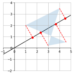
设置投影轴为倾斜的
angle30 = 30 * np.pi / 180  # angle in radians
U_30 = np.array([[np.cos(angle30), np.sin(angle30)]])
plot_projection(U_30, P)

这里要仔细分析一下,为什么是往
直线上投影(这里
)
我们回顾下投影的表达式
当
是单位向量的时候,
为1,所以公式可以进一步化简为
总结:向量 往单位向量 上投影的模长就等于该向量与单位向量的内积(inner product),投影的方向同单位向量的方向!
所以,我们用矩阵 U_30 = np.array([[np.cos(angle30), np.sin(angle30)]]) 乘以原来的矩阵,对应到矩阵的每一列,也就是每一个坐标的话,相当于每个列向量往 U_30 上投影

这样对比着看就显而易见了,嘿嘿嘿!(上面右图是在 def plot_projection 函数中添加如下代码的结果)
def plot_projection(U, P):
	#………
    # 画向量
    for i in range(np.shape(P)[1]):#遍历所
        plot_vector2d(P[:,i],color="r")
3.3.2 Rotation
现在探究下用 2*2 矩阵,2*2 乘以原来的 2*4,结果还是 2*4
修改下 def plot_projection(U, P): 函数
- 把坐标轴的尺度统一(正方形,而不是长方形)
- 画个坐标轴
%matplotlib inline
import matplotlib.pyplot as plt
import numpy as np
from matplotlib.patches import Polygon

def plot_projection(U, P):
    U_P = U.dot(P)

    # 投影轴
    axis_end = 100 * U
    plot_vector2d(axis_end[0], color="black")
    plot_vector2d(-axis_end[0], color="black")

    # 画矩阵
    plt.gca().add_artist(Polygon(P.T, alpha=0.2))

    for vector, proj_coordinate in zip(P.T, U_P.T):
        proj_point = proj_coordinate * U # 投影后的矢量 U.dot(P) * U
        plt.plot(proj_point[0][0], proj_point[0][1], "ro") # 画点 [[]]
        plt.plot([vector[0], proj_point[0][0]], [vector[1], proj_point[0][1]], "r--") # 画 [x0,x1],[y0,y1]

    plt.axis([-1, 5, -2, 4])

    # 画 x 轴和 y 轴
    ax = plt.gca() # x,y
    # spines = 上下左右四条黑线
    ax.spines['right'].set_color('none') # 让右边的黑线消失
    ax.spines['top'].set_color('none')  # 让上边的黑线消失
    ax.xaxis.set_ticks_position('bottom') # 把下面的黑线设置为x轴
    ax.yaxis.set_ticks_position('left')   #  把左边的黑线设置为y轴
    ax.spines['bottom'].set_position(('data',0)) # 移动x轴到指定位置,本例子为0
    ax.spines['left'].set_position(('data',0))   # 移动y轴到指定位置,本例子为0

    # 设置 x 轴和 y 轴等距
    plt.gca().set_aspect('equal', adjustable='box')
    plt.grid()
    plt.show()
我们用以下矩阵来乘以原来的 矩阵!
也即
有了前面投影的基础,我们可以理解为,新的横坐标的绝对值是原来的点往
的直线上投影的模长,新的纵坐标的绝对值是原来的点往
的直线上投影的模长!
P = np.array([
        [3.0, 4.0, 1.0, 4.6],
        [0.2, 3.5, 2.0, 0.5]
    ]) # 2,4

angle30 = 30 * np.pi / 180  # angle in radians
U_30 = np.array([[np.cos(angle30), np.sin(angle30)]])
plot_projection(U_30, P)

angle120 = 120 * np.pi / 180  # angle in radians
U_120 = np.array([[np.cos(angle120), np.sin(angle120)]])
plot_projection(U_120, P)
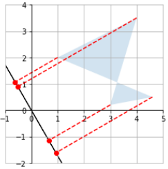
我们来看一下联合在一起的效果!!!
%matplotlib inline
import matplotlib.pyplot as plt
import numpy as np
from matplotlib.patches import Polygon
import numpy.linalg as LA

def cal_theta(P,P_rotated):
    theta = [] # 存放每个坐标的角度变换
    for i in range(P_rotated.shape[1]):#遍历每一列
        radian = P[:,i].dot(P_rotated[:,i]) / (LA.norm(P[:,i])*LA.norm(P_rotated[:,i])) # 计算弧度
        theta.append(radian*180/np.pi) #转化为角度
    return theta

P = np.array([
        [3.0, 4.0, 1.0, 4.6],
        [0.2, 3.5, 2.0, 0.5]
    ]) # 2,4

angle30 = 30 * np.pi / 180  # angle in radians
angle120 = 120 * np.pi / 180  # angle in radians

V = np.array([
        [np.cos(angle30), np.sin(angle30)],
        [np.cos(angle120), np.sin(angle120)]
    ])

P_rotated = V.dot(P)

theta = cal_theta(P,P_rotated)
print(theta)

plot_transformation(P, P_rotated, "$P$", "$VP$", [-1, 7, -1, 5], arrows=True)
plt.show()
其中 def plot_transformation 见 3.2 小节 Scalar Multiplication
output
[49.61960058796129, 49.61960058796129, 49.61960058796129, 49.61960058796128]

哈哈哈,大吃一惊,怎么是顺时针移动了
,把投影换成负数试试
angle30 = 30 * np.pi / 180  # angle in radians
angle120 = 120 * np.pi / 180  # angle in radians
改为
angle30 = -30 * np.pi / 180  # angle in radians
angle120 = 60 * np.pi / 180  # angle in radians
output
[49.61960058796129, 49.61960058796129, 49.61960058796129, 49.61960058796128]

逆时针转动了
之前我们保持了横纵坐标的变化的差值为 ,这样形状就不会变化!下面试试别的
3.3.3 Shear
P = np.array([
        [3.0, 4.0, 1.0, 4.6],
        [0.2, 3.5, 2.0, 0.5]
    ]) # 2,4

F_shear = np.array([
        [1, 1.5],
        [0, 1]
    ])
plot_transformation(P, F_shear.dot(P), "$P$", "$F_{shear} P$",
                    axis=[0, 10, 0, 7])
plt.show()
其中 def plot_transformation 见 3.2 小节 Scalar Multiplication

看看作用在方阵上的效果
F_shear = np.array([
        [1, 1.5],
        [0, 1]
    ])

Square = np.array([
        [0, 0, 1, 1],
        [0, 1, 1, 0]
    ])
plot_transformation(Square, F_shear.dot(Square), "$Square$", "$F_{shear} Square$",
                    axis=[0, 2.6, 0, 1.8])
plt.show()
1)偏离 0.5 和 1.0
F_shear = np.array([
        [1, 0.5],
        [0, 1]
    ])
F_shear = np.array([
        [1, 1.0],
        [0, 1]
    ])


2)偏离 1.5 和 -0.5
F_shear = np.array([
        [1, 1.5],
        [0, 1]
    ])
F_shear = np.array([
        [1, -0.5],
        [0, 1]
    ])


3)纵坐标偏离
F_shear = np.array([
        [1, 0],
        [0.5, 1]
    ])

4)一起来
F_shear = np.array([
        [1, 0.5],
        [0.5, 1]
    ])

3.3.4 Squeeze
P = np.array([
        [3.0, 4.0, 1.0, 4.6],
        [0.2, 3.5, 2.0, 0.5]
    ]) # 2,4

F_squeeze = np.array([
        [1.2, 0],
        [0, 1/1.2]
    ])
plot_transformation(P, F_squeeze.dot(P), "$P$", "$F_{squeeze} P$",
                    axis=[0, 7, 0, 5])
plt.show()
其中 def plot_transformation 见 3.2 小节 Scalar Multiplication

F_squeeze = np.array([
        [1.5, 0],
        [0, 1/1.5]
    ])
增大后发现压缩的更用力

如果参数一样,就是缩放功能了
F_squeeze = np.array([
        [1.5, 0],
        [0, 1.5]
    ])

3.3.5 Flip
1)Vertical flip
F_reflect = np.array([
        [1, 0],
        [0, -1]
    ])
plot_transformation(P, F_reflect.dot(P), "$P$", "$F_{reflect} P$",
                    axis=[-2, 9, -4.5, 4.5])
plt.show()
其中 def plot_transformation 见 3.2 小节 Scalar Multiplication

2)Horizental flip
F_reflect = np.array([
        [-1, 0],
        [0, 1]
    ])
plot_transformation(P, F_reflect.dot(P), "$P$", "$F_{reflect} P$",
                    axis=[-6, 6, 0, 6])
plt.show()

3)中心对称
F_reflect = np.array([
        [-1, 0],
        [0, -1]
    ])
plot_transformation(P, F_reflect.dot(P), "$P$", "$F_{reflect} P$",
                    axis=[-5, 5, -3.5, 3.5])
plt.show()

3.4 Matrix Inverse
逆矩阵的求法如下
import numpy as np
import numpy.linalg as LA

F_shear = np.array([
        [1, 1.5],
        [0, 1]
    ])
F_inv_shear = LA.inv(F_shear)
F_inv_shear
output
array([[ 1. , -1.5],
       [ 0. ,  1. ]])
接下来探讨下逆矩阵的魅力
P = np.array([
        [3.0, 4.0, 1.0, 4.6],
        [0.2, 3.5, 2.0, 0.5]
    ]) # 2,4

F_shear = np.array([
        [1, 1.5],
        [0, 1]
    ])

F_inv_shear = np.array([
    [1, -1.5],
    [0, 1]
])

print(F_shear.dot(F_inv_shear),'\n')
print(F_inv_shear.dot(F_shear))

# 原矩阵和逆矩阵相乘为I
P_sheared = F_shear.dot(P)
P_unsheared = F_inv_shear.dot(P_sheared)

plot_transformation(P_sheared, P_unsheared, "$P_{sheared}$", "$P_{unsheared}$",
                    axis=[0, 10, 0, 7])
plt.plot(P[0], P[1], "b--") # set[x],set[y],画虚线
plt.show()
其中 def plot_transformation 见 3.2 小节 Scalar Multiplication
output
[[1. 0.]
 [0. 1.]]

[[1. 0.]
 [0. 1.]]

蓝色虚线表示原来的矩阵,可以看到,左乘 shear 之后,然后再左乘 shear 的逆,图形没有任何变化,这是因为
然后单位矩阵乘以任何矩阵结果都是任何矩阵本身!
3.5 Determinant
import numpy as np
import numpy.linalg as LA
M = np.array([
        [1, 2, 3],
        [4, 5, 6],
        [7, 8, 0]
    ])
LA.det(M)
output
27.0
P = np.array([
        [3.0, 4.0, 1.0, 4.6],
        [0.2, 3.5, 2.0, 0.5]
    ]) # 2,4

F_scale = np.array([
        [0.5, 0],
        [0, 0.5]
    ])
plot_transformation(P, F_scale.dot(P), "$P$", "$F_{scale} \cdot P$",
                    axis=[0, 6, -1, 4])
plt.show()
其中 def plot_transformation 见 3.2 小节 Scalar Multiplication

P = np.array([
        [3.0, 4.0, 1.0, 4.6],
        [0.2, 3.5, 2.0, 0.5]
    ]) # 2,4

F_flip = np.array([
        [-1, 0],
        [0, 1]
    ])
plot_transformation(P, F_flip.dot(P), "$P$", "$F_{Flip} \cdot P$",
                    axis=[-6, 6, 0, 6])
plt.show()

LA.det(F_flip)
结果是 -1.0
对角矩阵的特征值等于对角线上的元素,而行列式的值等于特征值的乘积!
3.6 Singular Value Decomposition(SVD)
关于 SVD 的数学推导可以参考 Singular Value Decomposition
import numpy as np
import numpy.linalg as LA

F_shear = np.array([
        [1, 1.5],
        [0, 1]
    ])
# 对 F_shear 矩阵进行 SVD
U, S_diag, V_T = LA.svd(F_shear)
print(U,'\n')
print(S_diag,'\n')
print(V_T,'\n')

# 返回的是主对角线的元素,我们把它变成对角矩阵
S = np.diag(S_diag)
print(S)
output
[[ 0.89442719 -0.4472136 ]
 [ 0.4472136   0.89442719]]

[2.  0.5]

[[ 0.4472136   0.89442719]
 [-0.89442719  0.4472136 ]]

[[2.  0. ]
 [0.  0.5]]
我们还原回去试试
U.dot(np.diag(S_diag)).dot(V_T)
output
array([[1. , 1.5],
       [0. , 1. ]])
nice,和 F_shear 矩阵一样,F_shear 作用在方阵的效果如下:
Square = np.array([
        [0, 0, 1, 1],
        [0, 1, 1, 0]
    ])
plot_transformation(Square, F_shear.dot(Square), "$Square$", "$F_{shear} Square$",
                    axis=[-0.5, 3.5 , -1.5, 1.5])
plt.show()
其中 def plot_transformation 见 3.2 小节 Scalar Multiplication

接下来我们看看 SVD 分解后每一个部分的作用!
1)首先是
plot_transformation(Square, V_T.dot(Square), "$Square$", "$V^T \cdot Square$",
                    axis=[-0.5, 3.5 , -1.5, 1.5])
plt.show()

2)再是
plot_transformation(V_T.dot(Square), S.dot(V_T).dot(Square), "$V^T \cdot Square$", "$\Sigma \cdot V^T \cdot Square$",
                    axis=[-0.5, 3.5 , -1.5, 1.5])
plt.show()

3)最后是
plot_transformation(S.dot(V_T).dot(Square), U.dot(S).dot(V_T).dot(Square),"$\Sigma \cdot V^T \cdot Square$", "$U \cdot \Sigma \cdot V^T \cdot Square$",
                    axis=[-0.5, 3.5 , -1.5, 1.5])
plt.show()

And we can see that the result is indeed a shear mapping of the original unit square.
3.7 Eigenvectors and Eigenvalues
import numpy as np
import numpy.linalg as LA
A = np.array([
        [1, 1, 0],
        [1, 2, 1],
        [0, 1, 1],
    ])

eigenvalues, eigenvectors = LA.eig(A)

print(eigenvalues,'\n')
print(eigenvectors)
output
[ 3.00000000e+00  1.00000000e+00 -3.36770206e-17]

[[-4.08248290e-01  7.07106781e-01  5.77350269e-01]
 [-8.16496581e-01  2.61239546e-16 -5.77350269e-01]
 [-4.08248290e-01 -7.07106781e-01  5.77350269e-01]]
可以对比下 Singular Value Decomposition 的一个例子的结果
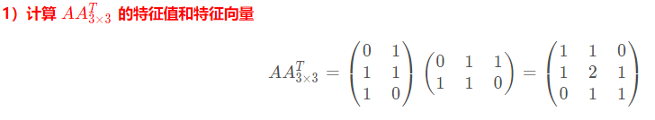
特征值为 3,1,0,对应的特征向量如下
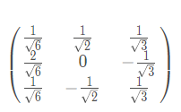
试试
from math import sqrt
print(1/sqrt(6))
print(1/sqrt(2))
print(1/sqrt(3))
output
0.4082482904638631
0.7071067811865475
0.5773502691896258
没有问题,哈哈,不过好像不能表示 0
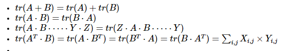
3.8 Trace
等于对角线上元素的和
import numpy as np
import numpy.linalg as LA
D = np.array([
        [100, 200, 300],
        [ 10,  20,  30],
        [  1,   2,   3],
    ])
np.trace(D)
结果为 123