▶ 使用 Ada Boosting 方法提升若干个弱分类器的效果
● 代码,每个感知机仅训练原数据集 trainRatio = 30% 的数据,然后进行调整和提升
  1 import numpy as np
  2 import matplotlib.pyplot as plt
  3 from mpl_toolkits.mplot3d import Axes3D
  4 from mpl_toolkits.mplot3d.art3d import Poly3DCollection
  5 from matplotlib.patches import Rectangle
  6
  7 dataSize = 500
  8 trainDataRatio = 0.3
  9 ita = 0.3
 10 defaultTrainRatio = 0.3                                                         # 故意减少简单分类器的训练轮数
 11 randomSeed = 103
 12
 13 def myColor(x):                                                                 # 颜色函数
 14     r = np.select([x < 1/2, x < 3/4, x <= 1, True],[0, 4 * x - 2, 1, 0])
 15     g = np.select([x < 1/4, x < 3/4, x <= 1, True],[4 * x, 1, 4 - 4 * x, 0])
 16     b = np.select([x < 1/4, x < 1/2, x <= 1, True],[1, 2 - 4 * x, 0, 0])
 17     return [r**2,g**2,b**2]
 18
 19 def dataSplit(dataX, dataY, part):                                              # 将数据集分割为训练集和测试集
 20     return dataX[:part,:],dataY[:part], dataX[part:,:], dataY[part:]
 21
 22 def function(x,para):                                                           # 连续回归函数,用于画图
 23     return np.sum(x * para[0]) - para[1]                                        # 注意是减号
 24
 25 def judgeWeak(x, para):                                                         # 弱分类判别函数
 26     return np.sign(function(x, para))
 27
 28 def judgeStrong(x, paraList , alpha):                                           # 强分类判别函数,调用弱分类判别函数进行线性加和
 29     return np.sign( np.sum([ judgeWeak(x, paraList[i]) * alpha[i] for i in range(len(paraList)) ]) )
 30
 31 def targetIndex(x, xList):                                                      # 二分查找 xList 中不大于 x 的最大索引
 32     lp = 0
 33     rp = len(xList) - 1
 34     mp = mp = (lp + rp) >> 1
 35     while lp < mp:
 36         if(xList[mp] > x):
 37             rp = mp
 38         else:
 39             lp = mp
 40         mp = (lp + rp) >> 1
 41     return mp
 42
 43 def createData(dim, count = dataSize):                                          # 创建数据
 44     np.random.seed(randomSeed)
 45     X = np.random.rand(count, dim)
 46     if dim == 1:
 47         Y = (X > 0.5).astype(int).flatten() * 2 - 1
 48     else:
 49         Y = ((3 - 2 * dim) * X[:,0] + 2 * np.sum(X[:,1:], 1) > 0.5).astype(int) * 2 - 1
 50     print( "dim = %d, dataSize = %d, class1Ratio = %f"%(dim, count, np.sum((Y == 1).astype(int)) / count) )
 51     return X, Y
 52
 53 def perceptron(dataX, dataY, weight, trainRatio = defaultTrainRatio):           # 单层感知机,只训练 dataX 中占比为 trainRatio 的数据
 54     count, dim = np.shape(dataX)
 55     xE = np.concatenate((dataX, -np.ones(count)[:,np.newaxis]), axis = 1)
 56     w = np.zeros(dim + 1)
 57     accWeight = np.cumsum(weight)                                               # 累加分布列用于随机选取
 58     finishFlag = False
 59     for i in range(int(count * trainRatio)):
 60         j = targetIndex(np.random.rand(), accWeight)                            # 依分布列随机抽取一个样本进行训练
 61         w += ita * (dataY[j] - np.sign(np.sum(xE[j] * w))) * xE[j]
 62     return (w[:-1],w[-1])
 63
 64 def adaBoost(dataX, dataY, weakCount):                                          # 提升训练
 65     count, dim = np.shape(dataX)
 66     weight = np.ones(count) / count                                             # 样本权重
 67     paraList = []                                                               # 弱分类器的系数
 68     alpha = np.zeros(weakCount)                                                 # 弱分类器的权重
 69     for i in range(weakCount):
 70         para = perceptron(dataX, dataY, weight)                                 # 每次训练后检查训练集的分类情况,调整弱分类器权重和样本权重
 71         trainResult = [ judgeWeak(i, para) for i in dataX ]
 72         trainErrorRatio = np.sum( (np.array(trainResult) != dataY).astype(int) * weight )
 73         paraList.append(para)
 74         alpha[i] = np.log(1 / (trainErrorRatio + 1e-8) - 1) / 2
 75         weight *= np.exp( -alpha[i] * dataY * trainResult )
 76         weight /= np.sum(weight)
 77     return paraList, alpha
 78
 79 def test(dim, weakCount):                                                       # 测试函数
 80     allX, allY = createData(dim)
 81     trainX, trainY, testX,testY = dataSplit(allX, allY, int(dataSize * trainDataRatio))
 82
 83     paraList, alpha = adaBoost(trainX, trainY, weakCount)
 84
 85     testResult = [ judgeStrong(i, paraList, alpha) for i in testX ]
 86     errorRatio = np.sum( (np.array(testResult) != testY).astype(int)**2 ) / (dataSize*(1-trainDataRatio))
 87     print( "dim = %d, weakCount = %d, errorRatio = %f"%(dim, weakCount, round(errorRatio,4)) )
 88     for i in range(weakCount):
 89         print(alpha[i] , "\t\t", paraList[i])
 90
 91     if dim >= 4:                                                                # 4维以上不画图,只输出测试错误率
 92         return
 93
 94     classP = [ [],[] ]
 95     errorP = []
 96     for i in range(len(testX)):
 97         if testResult[i] != testY[i]:
 98             if dim == 1:
 99                 errorP.append(np.array([testX[i], int(testY[i]+1)>>1]))
100             else:
101                 errorP.append(np.array(testX[i]))
102         else:
103             classP[int(testResult[i]+1)>>1].append(testX[i])
104     errorP = np.array(errorP)
105     classP = [ np.array(classP[0]), np.array(classP[1]) ]
106
107     fig = plt.figure(figsize=(10, 8))
108     if dim == 1:
109         plt.xlim(0.0,1.0)
110         plt.ylim(-0.25,1.25)
111         for i in range(2):
112             if(len(classP[i])) > 0:
113                 plt.scatter(classP[i], np.ones(len(classP[i])) * i, color = myColor(i/2), s = 8, label = "class" + str(i))
114         if len(errorP) != 0:
115             plt.scatter(errorP[:,0], errorP[:,1],color = myColor(1), s = 16,label = "errorData")
116
117         plt.plot([0.5, 0.5], [-0.25, 1.25], color = [0.5,0.25,0],label = "realBoundary")
118         plt.text(0.2, 1.1, "realBoundary: 2x = 1\nerrorRatio = " + str(round(errorRatio,4)),\
119             size=15, ha="center", va="center", bbox=dict(boxstyle="round", ec=(1., 0.5, 0.5), fc=(1., 1., 1.)))
120         R = [ Rectangle((0,0),0,0, color = myColor(i / 2)) for i in range(2) ] + [ Rectangle((0,0),0,0, color = myColor(1)), Rectangle((0,0),0,0, color = [0.5,0.25,0]) ]
121         plt.legend(R, [ "class" + str(i) for i in range(2) ] + ["errorData", "realBoundary"], loc=[0.81, 0.2], ncol=1, numpoints=1, framealpha = 1)
122
123     if dim == 2:
124         plt.xlim(-0.1, 1.1)
125         plt.ylim(-0.1, 1.1)
126         for i in range(2):
127             if(len(classP[i])) > 0:
128                 plt.scatter(classP[i][:,0], classP[i][:,1], color = myColor(i/2), s = 8, label = "class" + str(i))
129         if len(errorP) != 0:
130             plt.scatter(errorP[:,0], errorP[:,1], color = myColor(1), s = 16, label = "errorData")
131         plt.plot([0,1], [1/4,3/4], color = [0.5,0.25,0], label = "realBoundary")
132         plt.text(0.78, 1.02, "realBoundary: -x + 2y = 1\nerrorRatio = " + str(round(errorRatio,4)), \
133             size = 15, ha="center", va="center", bbox=dict(boxstyle="round", ec=(1., 0.5, 0.5), fc=(1., 1., 1.)))
134         R = [ Rectangle((0,0),0,0, color = myColor(i / 2)) for i in range(2) ] + [ Rectangle((0,0),0,0, color = myColor(1)) ]
135         plt.legend(R, [ "class" + str(i) for i in range(2) ] + ["errorData"], loc=[0.84, 0.012], ncol=1, numpoints=1, framealpha = 1)
136
137     if dim == 3:
138         ax = Axes3D(fig)
139         ax.set_xlim3d(0.0, 1.0)
140         ax.set_ylim3d(0.0, 1.0)
141         ax.set_zlim3d(0.0, 1.0)
142         ax.set_xlabel('X', fontdict={'size': 15, 'color': 'k'})
143         ax.set_ylabel('Y', fontdict={'size': 15, 'color': 'k'})
144         ax.set_zlabel('Z', fontdict={'size': 15, 'color': 'k'})
145         for i in range(2):
146             if(len(classP[i])) > 0:
147                 ax.scatter(classP[i][:,0], classP[i][:,1], classP[i][:,2], color = myColor(i/2), s = 8, label = "class" + str(i))
148         if len(errorP) != 0:
149             ax.scatter(errorP[:,0], errorP[:,1],errorP[:,2], color = myColor(1), s = 8, label = "errorData")
150         v = [(0, 0, 0.25), (0, 0.25, 0), (0.5, 1, 0), (1, 1, 0.75), (1, 0.75, 1), (0.5, 0, 1)]
151         f = [[0,1,2,3,4,5]]
152         poly3d = [[v[i] for i in j] for j in f]
153         ax.add_collection3d(Poly3DCollection(poly3d, edgecolor = 'k', facecolors = [0.5,0.25,0,0.5], linewidths=1))
154         ax.text3D(0.75, 0.92, 1.15, "realBoundary: -3x + 2y +2z = 1\nerrorRatio = " + str(round(errorRatio,4)), \
155             size = 12, ha="center", va="center", bbox=dict(boxstyle="round", ec=(1, 0.5, 0.5), fc=(1, 1, 1)))
156         R = [ Rectangle((0,0),0,0, color = myColor(i / 2)) for i in range(2) ] + [ Rectangle((0,0),0,0, color = myColor(1)) ]
157         plt.legend(R, [ "class" + str(i) for i in range(2) ] + ["errorData"], loc=[0.84, 0.012], ncol=1, numpoints=1, framealpha = 1)
158
159     fig.savefig("R:\\dim" + str(dim) + "kind2" + "weakCount" + str(weakCount) + ".png")
160     plt.close()
161
162 if __name__ == '__main__':
163     test(1, 1)                                                                  # 不同维数和弱分类器数的组合
164     test(1, 2)
165     test(1, 3)
166     test(1, 4)
167     test(2, 1)
168     test(2, 2)
169     test(2, 3)
170     test(2, 4)
171     test(3, 1)
172     test(3, 2)
173     test(3, 3)
174     test(3, 4)
175     test(4, 1)
176     test(4, 2)
177     test(4, 3)
178     test(4, 4)
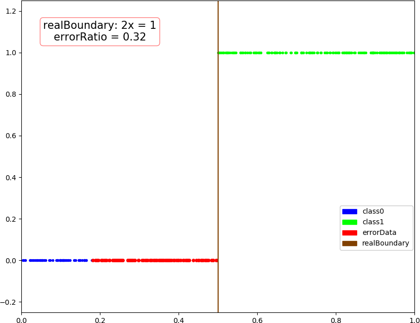
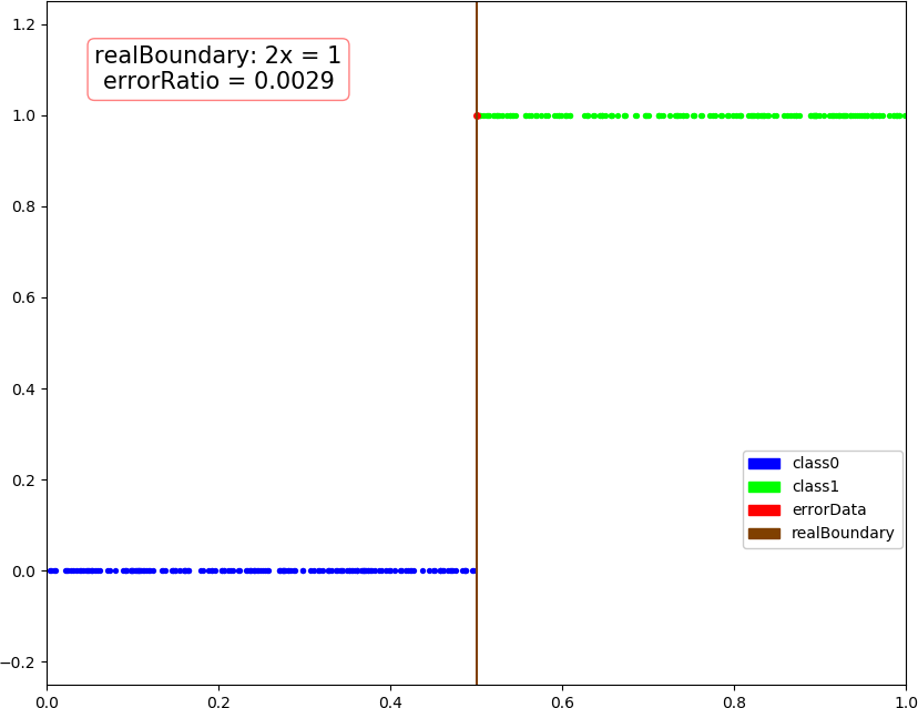
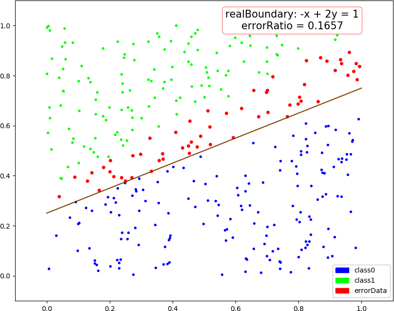
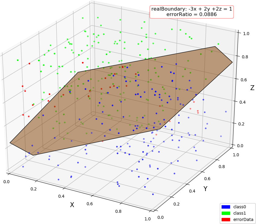
● 输出结果,随着使用的弱分类器数量的增多,预测精度逐渐上升。低维情况不明显,少数的弱分类器就已经达到了较好的精度,高维情况中,精度上升会抖动,被分类的点在分类结果中也会抖动。
dim = 1, dataSize = 500, class1Ratio = 0.492000
dim = 1, weakCount = 1, errorRatio = 0.320000
0.34657356777997284              (array([1.67141915]), 0.29999999999999993)
dim = 1, dataSize = 500, class1Ratio = 0.492000
dim = 1, weakCount = 2, errorRatio = 0.002900
0.34657356777997284              (array([1.67141915]), 0.29999999999999993)
2.6466513960316105               (array([0.59811356]), 0.3)
dim = 1, dataSize = 500, class1Ratio = 0.492000
dim = 1, weakCount = 3, errorRatio = 0.002900
0.34657356777997284              (array([1.67141915]), 0.29999999999999993)
2.6466513960316105               (array([0.59811356]), 0.3)
1.154062035731127                (array([0.70689064]), 0.29999999999999993)
dim = 1, dataSize = 500, class1Ratio = 0.492000
dim = 1, weakCount = 4, errorRatio = 0.002900
0.34657356777997284              (array([1.67141915]), 0.29999999999999993)
2.6466513960316105               (array([0.59811356]), 0.3)
1.154062035731127                (array([0.70689064]), 0.29999999999999993)
0.41049029622924904              (array([0.65816408]), 0.29999999999999993)
dim = 2, dataSize = 500, class1Ratio = 0.520000
dim = 2, weakCount = 1, errorRatio = 0.165700
0.7581737108087062               (array([-0.5342485 ,  0.85301855]), 0.3)
dim = 2, dataSize = 500, class1Ratio = 0.520000
dim = 2, weakCount = 2, errorRatio = 0.140000
0.7581737108087062               (array([-0.5342485 ,  0.85301855]), 0.3)
1.1603017192470149               (array([-0.23046473,  1.17772171]), 0.29999999999999993)
dim = 2, dataSize = 500, class1Ratio = 0.520000
dim = 2, weakCount = 3, errorRatio = 0.082900
0.7581737108087062               (array([-0.5342485 ,  0.85301855]), 0.3)
1.1603017192470149               (array([-0.23046473,  1.17772171]), 0.29999999999999993)
1.366866794214113                (array([-0.86403595,  1.29893022]), 0.3)
dim = 2, dataSize = 500, class1Ratio = 0.520000
dim = 2, weakCount = 4, errorRatio = 0.082900
0.7581737108087062               (array([-0.5342485 ,  0.85301855]), 0.3)
1.1603017192470149               (array([-0.23046473,  1.17772171]), 0.29999999999999993)
1.366866794214113                (array([-0.86403595,  1.29893022]), 0.3)
-0.07595124913479236             (array([-0.71435958,  1.09996259]), 0.3)
dim = 3, dataSize = 500, class1Ratio = 0.544000
dim = 3, weakCount = 1, errorRatio = 0.334300
0.4236489063840784               (array([-1.88583778,  1.00159772,  0.23076269]), 0.3)
dim = 3, dataSize = 500, class1Ratio = 0.544000
dim = 3, weakCount = 2, errorRatio = 0.097100
0.4236489063840784               (array([-1.88583778,  1.00159772,  0.23076269]), 0.3)
1.2147383422658522               (array([-1.11207425,  0.87462922,  1.16116403]), 0.29999999999999993)
dim = 3, dataSize = 500, class1Ratio = 0.544000
dim = 3, weakCount = 3, errorRatio = 0.074300
0.4236489063840784               (array([-1.88583778,  1.00159772,  0.23076269]), 0.3)
1.2147383422658522               (array([-1.11207425,  0.87462922,  1.16116403]), 0.29999999999999993)
1.4030555888409086               (array([-0.90813279,  0.97916935,  0.44726373]), 0.3)
dim = 3, dataSize = 500, class1Ratio = 0.544000
dim = 3, weakCount = 4, errorRatio = 0.088600
0.4236489063840784               (array([-1.88583778,  1.00159772,  0.23076269]), 0.3)
1.2147383422658522               (array([-1.11207425,  0.87462922,  1.16116403]), 0.29999999999999993)
1.4030555888409086               (array([-0.90813279,  0.97916935,  0.44726373]), 0.3)
0.298249916659031                (array([-0.92372522,  1.11109598,  0.9864088 ]), -0.30000000000000004)
dim = 4, weakCount = 1, errorRatio = 0.271400
0.6328331575281093               (array([-1.55413592,  1.59665079,  0.46795061,  1.01271949]), 0.29999999999999993)
dim = 4, dataSize = 500, class1Ratio = 0.484000
dim = 4, weakCount = 2, errorRatio = 0.271400
0.6328331575281093               (array([-1.55413592,  1.59665079,  0.46795061,  1.01271949]), 0.29999999999999993)
0.4566505516305031               (array([-2.06478282, -0.07030723,  0.28072944,  0.50215833]), 0.30000000000000004)
dim = 4, dataSize = 500, class1Ratio = 0.484000
dim = 4, weakCount = 3, errorRatio = 0.271400
0.6328331575281093               (array([-1.55413592,  1.59665079,  0.46795061,  1.01271949]), 0.29999999999999993)
0.4566505516305031               (array([-2.06478282, -0.07030723,  0.28072944,  0.50215833]), 0.30000000000000004)
0.1788001854725199               (array([-1.57793113,  1.11981   ,  0.68428309,  0.48606427]), -0.3)
dim = 4, dataSize = 500, class1Ratio = 0.484000
dim = 4, weakCount = 4, errorRatio = 0.177100
0.6328331575281093               (array([-1.55413592,  1.59665079,  0.46795061,  1.01271949]), 0.29999999999999993)
0.4566505516305031               (array([-2.06478282, -0.07030723,  0.28072944,  0.50215833]), 0.30000000000000004)
0.1788001854725199               (array([-1.57793113,  1.11981   ,  0.68428309,  0.48606427]), -0.3)
0.8838043587493469               (array([-1.46314889,  0.7044062 ,  0.47142833,  0.2926442 ]), 0.3)
● 画图,行:数据维数,列:分别使用 1 ~ 4 个弱分类器