这个问题是我在SLAM求职宝典系列D2篇中遗留的问题,因为内容较多现在单独将其列出进行解答。
本篇内容分为四个部分:
目录
(4) OpenCV中连通域的求解(C++ & Python)
(1)二值图
二值图像,顾名思义就是图像的亮度值只有两个状态:黑(0)和白(255)。二值图像在图像分析与识别中有着举足轻重的地位,因为其模式简单,对像素在空间上的关系有着极强的表现力。在实际应用中,很多图像的分析最终都转换为二值图像的分析,比如:医学图像分析、前景检测、字符识别,形状识别。二值化+数学形态学能解决很多计算机识别工程中目标提取的问题。
举个例子如下图:

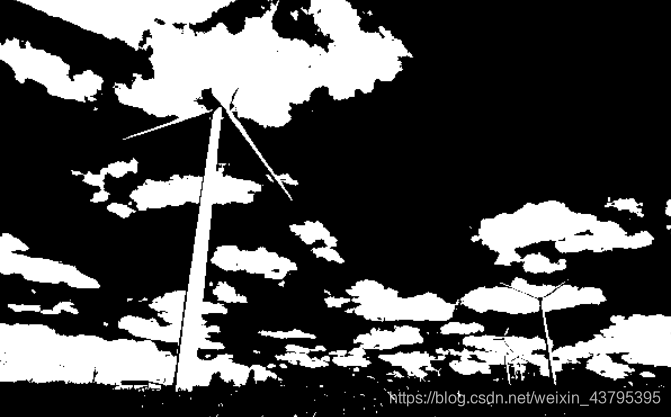
二值图像分析最重要的方法就是连通区域标记,它是所有二值图像分析的基础,它通过对二值图像中白色像素(目标)的标记,让每个单独的连通区域形成一个被标识的块,进一步的我们就可以获取这些块的轮廓、外接矩形、质心、不变矩等几何参数。
(2)求最大连通区域的算法
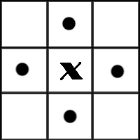
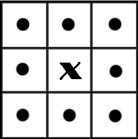
连通区域的定义有8点法和4点法,区别在于构成像素连通关系的邻接像素位置不一样。如下图,在图像中,最小的单位是像素,每个像素周围有8个邻接像素,常见的邻接关系有2种:4邻接与8邻接。4邻接一共4个点,即上下左右。8邻接的点一共有8个,包括了对角线位置的点。
连通具有传递性,如果A与B连通,B与C连通,则A与C也连通。
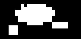
下面这符图中,如果考虑4邻接,则有3个连通区域;如果考虑8邻接,则有2个连通区域。
上面我们已经介绍了二值图的概念,黑白相的灰度值分别为0和255,但实际的考察中经常会简化为了0-1图,即图像中的数字是0或1 。
从连通区域的定义可以知道,一个连通区域是由具有相同像素值的相邻像素组成像素集合,因此,我们就可以通过这两个条件在图像中寻找连通区域,对于找到的每个连通区域,我们赋予其一个唯一的标识(Label),以区别其他连通区域。
连通区域分析有基本的算法,也有其改进算法,再谈到DFS和BFS之前,我们先来看一下求连通域经典的算法,这里列举两个常见的算法: 1)Two-Pass法; 2)Seed-Filling种子填充法
两遍扫描法 ——
Two-Pass算法的步骤:
1. 第一次扫描:
访问当前像素B(x,y),如果B(x,y) == 1:
(1)如果B(x,y)的领域中像素值都为0,则赋予B(x,y)一个新的label:
label += 1, B(x,y) = label;
(2)如果B(x,y)的领域中有像素B(x, y) > 1 的像素Neighbors:
a、将Neighbors中的最小值赋予给B(x,y):
B(x,y) = min{ Neighbors }
b、记录Neighbors中各个值(label)之间的相等关系,即这些值(label)同属同一个连通区域;
labelSet[i] = { label_m, .., label_n },labelSet[i]中的所有label都属于同一个连通区域 (注:这里可以有多种实现方式,只要能够记录这些具有相等关系的label之间的关系即可)
2. 第二次扫描:
访问当前像素B(x,y),如果B(x,y) > 1:
找到与label = B(x,y)同属相等关系的一个最小label值,赋予给B(x,y);
完成扫描后,图像中具有相同label值的像素就组成了同一个连通区域。
动图展示:

种子填充法——
种子填充方法来源于计算机图形学,常用于对某个图形进行填充。思路:选取一个前景像素点作为种子,然后根据连通区域的两个基本条件(像素值相同、位置相邻)将与种子相邻的前景像素合并到同一个像素集合中,最后得到的该像素集合则为一个连通区域。
下面给出基于种子填充法的连通区域分析方法:
1. 扫描图像,直到当前像素点B(x,y) == 1:
a、将B(x,y)作为种子(像素位置),并赋予其一个label,然后将该种子相邻的所有前景像素都压入栈中;
b、弹出栈顶像素,赋予其相同的label,然后再将与该栈顶像素相邻的所有前景像素都压入栈中;
c、重复b步骤,直到栈为空;
此时,便找到了图像B中的一个连通区域,该区域内的像素值被标记为label;
2. 重复第1步,直到扫描结束;
扫描结束后,就可以得到图像B中所有的连通区域;
动图展示:

这里的算法你会发现,实际上就是深度优先搜索的原理,我在slam求职程序基础(A)篇中,有介绍过树的深度优先和广度优先遍历,从那个例子中你可以看到一般我们用栈的数据结构来实现DFS, 用队列的数据结构来实现BFS。
那么这道题中所说的需要我们分别用DFS和BFS来实现,自然是指在种子填充法的这个框架下,对于一个连通域,从第一个种子出发我们可以用DFS来找到剩下的连通像素,稍加改动同样的任务,我们也可以用BFS来实现。和树的两种遍历其实是一个道理。
(3)代码实现,以及DFS 和 BFS
下面的代码参考其他博客,整理而成,另外加入了DFS和BFS的内容, 包含了不同方法以及主程序,较长。
如果你觉得厌倦,只想学习一下DFS和BFS,强烈建议看一下我的博客-SLAM、三维视觉求职宝典 | 程序基础篇(A)中的第13问题。
#include <iostream>
#include <string>
#include <list>
#include <vector>
#include <map>
#include <stack>
#include <opencv2/core/core.hpp>
#include <opencv2/highgui/highgui.hpp>
#include <opencv2/imgproc/imgproc.hpp>


using namespace std;
using namespace cv;


//------------------------------【两步法】----------------------------------------------
// 对二值图像进行连通区域标记,从1开始标号
void  Two_PassNew( const Mat &bwImg, Mat &labImg )
{
	assert( bwImg.type()==CV_8UC1 );
	labImg.create( bwImg.size(), CV_32SC1 );   //bwImg.convertTo( labImg, CV_32SC1 );
	labImg = Scalar(0);
	labImg.setTo( Scalar(1), bwImg );
	assert( labImg.isContinuous() );
	const int Rows = bwImg.rows - 1, Cols = bwImg.cols - 1;
	int label = 1;
	vector<int> labelSet;
	labelSet.push_back(0);
	labelSet.push_back(1);
	//the first pass
	int *data_prev = (int*)labImg.data;   //0-th row : int* data_prev = labImg.ptr<int>(i-1);
	int *data_cur = (int*)( labImg.data + labImg.step ); //1-st row : int* data_cur = labImg.ptr<int>(i);
	for( int i = 1; i < Rows; i++ )
	{
		data_cur++;
		data_prev++;
		for( int j=1; j<Cols; j++, data_cur++, data_prev++ )
		{
			if( *data_cur!=1 )
				continue;
			int left = *(data_cur-1);
			int up = *data_prev;
			int neighborLabels[2];
			int cnt = 0;
			if( left>1 )
				neighborLabels[cnt++] = left;
			if( up > 1)
				neighborLabels[cnt++] = up;
			if( !cnt )
			{
				labelSet.push_back( ++label );
				labelSet[label] = label;
				*data_cur = label;
				continue;
			}
			int smallestLabel = neighborLabels[0];
			if( cnt==2 && neighborLabels[1]<smallestLabel )
				smallestLabel = neighborLabels[1];
			*data_cur = smallestLabel;
			// 保存最小等价表
			for( int k=0; k<cnt; k++ )
			{
				int tempLabel = neighborLabels[k];
				int& oldSmallestLabel = labelSet[tempLabel];  //这里的&不是取地址符号,而是引用符号
				if( oldSmallestLabel > smallestLabel )
				{
					labelSet[oldSmallestLabel] = smallestLabel;
					oldSmallestLabel = smallestLabel;
				}
				else if( oldSmallestLabel<smallestLabel )
					labelSet[smallestLabel] = oldSmallestLabel;
			}
		}
		data_cur++;
		data_prev++;
	}
	//更新等价队列表,将最小标号给重复区域
	for( size_t i = 2; i < labelSet.size(); i++ )
	{
		int curLabel = labelSet[i];
		int prelabel = labelSet[curLabel];
		while( prelabel != curLabel )
		{
			curLabel = prelabel;
			prelabel = labelSet[prelabel];
		}
		labelSet[i] = curLabel;
	}
	//second pass
	data_cur = (int*)labImg.data;
	for( int i = 0; i < Rows; i++ )
	{
		for( int j = 0; j < bwImg.cols-1; j++, data_cur++)
			*data_cur = labelSet[ *data_cur ];
		data_cur++;
	}
}


//-------------------------------------------【种子填充法】---------------------------
void SeedFillNew(const cv::Mat& _binImg, cv::Mat& _lableImg )
{
	// connected component analysis(4-component)
	// use seed filling algorithm
	// 1. begin with a forgeground pixel and push its forground neighbors into a stack;
	// 2. pop the pop pixel on the stack and label it with the same label until the stack is empty
	//
	//  forground pixel: _binImg(x,y)=1
	//  background pixel: _binImg(x,y) = 0


	if(_binImg.empty() ||
		_binImg.type()!=CV_8UC1)
	{
		return;
	}

	_lableImg.release();
	_binImg.convertTo(_lableImg,CV_32SC1);

	int label = 0; //start by 1

	int rows = _binImg.rows;
	int cols = _binImg.cols;

	Mat mask(rows, cols, CV_8UC1);
	mask.setTo(0);
	int *lableptr;
	for(int i=0; i < rows; i++)
	{
		int* data = _lableImg.ptr<int>(i);
		uchar *masKptr = mask.ptr<uchar>(i);
		for(int j = 0; j < cols; j++)
		{
			if(data[j] == 255&&mask.at<uchar>(i,j)!=1)
			{
				mask.at<uchar>(i,j)=1;
				std::stack<std::pair<int,int>> neighborPixels;
				neighborPixels.push(std::pair<int,int>(i,j)); // pixel position: <i,j>
				++label; //begin with a new label
				while(!neighborPixels.empty())
				{
					//get the top pixel on the stack and label it with the same label
					std::pair<int,int> curPixel =neighborPixels.top();
					int curY = curPixel.first;
					int curX = curPixel.second;
					_lableImg.at<int>(curY, curX) = label;

					//pop the top pixel
					neighborPixels.pop();

					//push the 4-neighbors(foreground pixels)

					if(curX-1 >= 0)
					{
						if(_lableImg.at<int>(curY,curX-1) == 255&&mask.at<uchar>(curY,curX-1)!=1) //leftpixel
						{
							neighborPixels.push(std::pair<int,int>(curY,curX-1));
							mask.at<uchar>(curY,curX-1)=1;
						}
					}
					if(curX+1 <=cols-1)
					{
						if(_lableImg.at<int>(curY,curX+1) == 255&&mask.at<uchar>(curY,curX+1)!=1)
							// right pixel
						{
							neighborPixels.push(std::pair<int,int>(curY,curX+1));
							mask.at<uchar>(curY,curX+1)=1;
						}
					}
					if(curY-1 >= 0)
					{
						if(_lableImg.at<int>(curY-1,curX) == 255&&mask.at<uchar>(curY-1,curX)!=1)
							// up pixel
						{
							neighborPixels.push(std::pair<int,int>(curY-1, curX));
							mask.at<uchar>(curY-1,curX)=1;
						}
					}
					if(curY+1 <= rows-1)
					{
						if(_lableImg.at<int>(curY+1,curX) == 255&&mask.at<uchar>(curY+1,curX)!=1)
							//down pixel
						{
							neighborPixels.push(std::pair<int,int>(curY+1,curX));
							mask.at<uchar>(curY+1,curX)=1;
						}
					}
				}
			}
		}
	}
}


//---------------------------------【颜色标记程序】-----------------------------------
//彩色显示
cv::Scalar GetRandomColor()
{
	uchar r = 255 * (rand()/(1.0 + RAND_MAX));
	uchar g = 255 * (rand()/(1.0 + RAND_MAX));
	uchar b = 255 * (rand()/(1.0 + RAND_MAX));
	return cv::Scalar(b,g,r);
}


void LabelColor(const cv::Mat& labelImg, cv::Mat& colorLabelImg)
{
	int num = 0;
	if (labelImg.empty() ||
		labelImg.type() != CV_32SC1)
	{
		return;
	}

	std::map<int, cv::Scalar> colors;

	int rows = labelImg.rows;
	int cols = labelImg.cols;

	colorLabelImg.release();
	colorLabelImg.create(rows, cols, CV_8UC3);
	colorLabelImg = cv::Scalar::all(0);

	for (int i = 0; i < rows; i++)
	{
		const int* data_src = (int*)labelImg.ptr<int>(i);
		uchar* data_dst = colorLabelImg.ptr<uchar>(i);
		for (int j = 0; j < cols; j++)
		{
			int pixelValue = data_src[j];
			if (pixelValue > 1)
			{
				if (colors.count(pixelValue) <= 0)
				{
					colors[pixelValue] = GetRandomColor();
					num++;
				}

				cv::Scalar color = colors[pixelValue];
				*data_dst++   = color[0];
				*data_dst++ = color[1];
				*data_dst++ = color[2];
			}
			else
			{
				data_dst++;
				data_dst++;
				data_dst++;
			}
		}
	}
	printf("color num : %d \n", num );
}

//------------------------------------------【测试主程序】--------------------------------
int main()
{

	cv::Mat binImage = cv::imread("ltc2.jpg", 0);
	//cv::threshold(binImage, binImage, 50, 1, CV_THRESH_BINARY);
	cv::Mat labelImg;
	double time;
	time= getTickCount();
	//对应四种方法,需要哪一种,则调用哪一种
	//Two_PassOld(binImage, labelImg);
	//Two_PassNew(binImage, labelImg);
	//SeedFillOld(binImage, labelImg);
	//SeedFillNew(binImage, labelImg);
	time = 1000*((double)getTickCount() - time)/getTickFrequency();
    cout<<std::fixed<<time<<"ms"<<endl;
	//彩色显示
	cv::Mat colorLabelImg;
	LabelColor(labelImg, colorLabelImg);
	cv::imshow("colorImg", colorLabelImg);
	//灰度显示
	cv::Mat grayImg;
	labelImg *= 10;
	labelImg.convertTo(grayImg, CV_8UC1);
	cv::imshow("labelImg", grayImg);
	double minval, maxval;
	minMaxLoc(labelImg,&minval,&maxval);
	cout<<"minval"<<minval<<endl;
	cout<<"maxval"<<maxval<<endl;
	cv::waitKey(0);
	return 0;
}
想说的都写在了代码中。
问题中让我们求解最大连通域,实际上我们所完成的是找出所有的连通区域并做了标记。 所以还需要计算每个连通域的面积并找出最大值。
(4) OpenCV中连通域的求解(C++ & Python)
除了自己手动实现连通区域的求解,OpenCV中当然也自带了连通域的算法 ,这里做简单的介绍。
void DefectsDetector::LargestConnecttedComponent(Mat srcImage, Mat &dstImage)
{
    Mat temp;
    Mat labels;
    srcImage.copyTo(temp);

    //1. 标记连通域
    int n_comps = connectedComponents(temp, labels, 4, CV_16U);
    vector<int> histogram_of_labels;
    for (int i = 0; i < n_comps; i++)//初始化labels的个数为0
    {
        histogram_of_labels.push_back(0);
    }

    int rows = labels.rows;
    int cols = labels.cols;
    for (int row = 0; row < rows; row++) //计算每个labels的个数
    {
        for (int col = 0; col < cols; col++)
        {
            histogram_of_labels.at(labels.at<unsigned short>(row, col)) += 1;
        }
    }
    histogram_of_labels.at(0) = 0; //将背景的labels个数设置为0

    //2. 计算最大的连通域labels索引
    int maximum = 0;
    int max_idx = 0;
    for (int i = 0; i < n_comps; i++)
    {
        if (histogram_of_labels.at(i) > maximum)
        {
            maximum = histogram_of_labels.at(i);
            max_idx = i;
        }
    }

    //3. 将最大连通域标记为1
    for (int row = 0; row < rows; row++)
    {
        for (int col = 0; col < cols; col++)
        {
            if (labels.at<unsigned short>(row, col) == max_idx)
            {
                labels.at<unsigned short>(row, col) = 255;
            }
            else
            {
                labels.at<unsigned short>(row, col) = 0;
            }
        }
    }

    //4. 将图像更改为CV_8U格式
    labels.convertTo(dstImage, CV_8U);
}
顺便学习一下, Python中opencv的用法——
主要使用了如下方法:
- 首先通过findContours函数找到二值图像中的所有边界(这块看需要调节里面的参数)
- 然后通过contourArea函数计算每个边界内的面积
- 最后通过fillConvexPoly函数将面积最大的边界内部涂成背景
import cv2
import numpy as np
import matplotlib.pyplot as plt
if __name__ == '__main__':
img = cv2.imread('bw.bmp')
gray = cv2.cvtColor(img, cv2.COLOR_BGR2GRAY)
#find contours of all the components and holes
gray_temp = gray.copy() #copy the gray image because function
#findContours will change the imput image into another
contours, hierarchy = cv2.findContours(gray_temp, cv2.RETR_TREE, cv2.CHAIN_APPROX_NONE)
#show the contours of the imput image
cv2.drawContours(img, contours, -1, (0, 255, 255), 2)
plt.figure('original image with contours'), plt.imshow(img, cmap = 'gray')
#find the max area of all the contours and fill it with 0
area = []
for i in xrange(len(contours)):
area.append(cv2.contourArea(contours[i]))
max_idx = np.argmax(area)
cv2.fillConvexPoly(gray, contours[max_idx], 0)
#show image without max connect components
plt.figure('remove max connect com'), plt.imshow(gray, cmap = 'gray')
plt.show()
本文所参考博客有:
https://blog.csdn.net/augusdi/article/details/9008921