Ceres Solver 自学

介绍
Hello Word
导数

数值导数（Numeric Derivatives）
分析导数（Analytic Derivatives）
关于更多导数（More About Derivatives）

Powell's Function
曲线拟合
鲁棒性曲线拟合

介绍

Ceres可以用来解受边界约束的非线性最小二乘问题，如
$\min_x \frac{1}{2} \sum_i \rho_i(\Vert f_i(x_{i_1}, ...,x_{i_k})\Vert^2) \quad s.t \quad l_j \leq x_j \leq \mu_j \tag{1}$
这一章我们将学习如何使用Ceres Solver解(1)问题。表达式 $\rho_i(\Vert f_i(x_{i_1}, ..., x_{i_k})\Vert^2)$ 是ResidualBock，其中 $f_i(.)$ 是CostFunction，它依赖参数块 $[x_{i_1},...,x_{x_k}]$ 。在大多数优化问题中，一小组标量出现在一起（例如参数块 $[x_{i_1},...,x_{x_k}]$ ）。例如，相机的位姿由3个标量组成的平移向量和4个标量组成的旋转（用四元数表示旋转）组成，其中涉及到额一小组标量叫做ParameterBlock，当然一个parameterBlock可以仅仅是一个参数， $l_j$ 和 $\mu_j$ 是参数块 $x_j$ 的边界约束。

$\rho_i$ 是一个LossFunction，一个LossFunction是一个标量函数，它用来减少非线性最小二乘中outliners的影响。
在特性的情况下，当 $\rho_i(x) =x$ ，也就是identity function, 同时 $l_j = - \infty$ ， $\mu_j = \infty$ ，我们得到更熟悉的非线性最小二乘问题。
$\frac{1}{2}\sum_i \Vert f_i(x_{i_1}, .., x_{i_k}\Vert^2) \tag{2}$

Hello Word

一开始，我们考虑下面的一个问题，找该函数的最小值
$\frac{1}{2} (10-x)^2$
这是一个简单额问题，它的最小值是当 $x=10$ 的时候取得最小值，但是这是使用Ceres解这个问题一个好的开始。

第一步写一个仿函数(functor)，它用来估计函数 $f(x)=10-x$

struct CostFunctor{
  template <typename T>
  bool operator() (const T* const x, T* residual) const {
   residual[0] = T(10.0) - x[0];
   return true;
 }
};

注意这里重要的是operator()是一个模板方法，它假设所有的输入和输出是T类型，模板的使用允许Ceres调用CostFunctor::operator<T>()，对于T=double时仅仅需要残差(residual)值，对于T=Jet时需要雅克比。在导数那一节我们将要讨论Ceres中提供的多种导数类型。

一旦我们有了计算参差函数(residual function)的方法，就可以使用它构造一个最小二乘问题，然后使用Ceres 求解。

int main(int argc, char** argv) {
  google::InitGoogleLogging(argv[0]);

  // 1. 设置变量初始值
  double initial_x = 5.0;
  double x = initial_x;

  // 2. 构建一个问题.
  Problem problem;

  // 3. 配置cost function并使用ceres提供的自动求导的方式求导
  CostFunction* cost_function =
      new AutoDiffCostFunction<CostFunctor, 1, 1>(new CostFunctor);
  problem.AddResidualBlock(cost_function, NULL, &x);

  // 4. 启动求解器
  Solver::Options options;
  options.linear_solver_type = ceres::DENSE_QR;
  options.minimizer_progress_to_stdout = true;
  Solver::Summary summary;
  Solve(options, &problem, &summary);

  std::cout << summary.BriefReport() << "\n";
  std::cout << "x : " << initial_x
            << " -> " << x << "\n";
  return 0;
}

AutoDiffCostFunction将CostFunctor作为输入，自动求导它并使用CostFunction作为接口。
编译和运行 examples/helloworld.cc将得到

iter      cost      cost_change  |gradient|   |step|    tr_ratio  tr_radius  ls_iter  iter_time  total_time
   0  4.512500e+01    0.00e+00    9.50e+00   0.00e+00   0.00e+00  1.00e+04       0    5.33e-04    3.46e-03
   1  4.511598e-07    4.51e+01    9.50e-04   9.50e+00   1.00e+00  3.00e+04       1    5.00e-04    4.05e-03
   2  5.012552e-16    4.51e-07    3.17e-08   9.50e-04   1.00e+00  9.00e+04       1    1.60e-05    4.09e-03
Ceres Solver Report: Iterations: 2, Initial cost: 4.512500e+01, Final cost: 5.012552e-16, Termination: CONVERGENCE
x : 5 -> 10

从 $x =5$ 开始，求解器在两次迭代后到达10。仔细的读者注意到这是一个线性问题，线性求解应该能到到达最佳的值。求解器的默认配置意在非线性问题，为了简单性，在这个例子中没有改变它。的确，使用Ceres可以在一次迭代后获取它的解。另外我们还注意在一次迭代后求解器就非常接近最佳值0。当我们谈到Ceres的收敛和参数配置时将深入探讨这些细节。

导数

像大多数优化包一样，Ceres Solver依赖于能够在任意参数值下估计目标函数中每个项的值和导数。正确有效地做法对于获得好结果至关重要。 Ceres Solver提供了许多方法。你已经看到其中一个 - 自动求导的例子examples/helloworld.cc

我们将要考虑其他的两种:分析和数值导数（Analytic and numeric derivatives）。

数值导数（Numeric Derivatives）

在一些情况下，不可能定义一个模板cost functor，例如，当残差的估计涉及到调用一个你不能控制的库函数时。在那种情况下可以使用数值求导。用户定义一个仿函数来计算残差值，然后构造一个NumericDiffCostFunction使用它。例如，对于 $f(x) = 10 -x$ 对应的仿函数是

struct NumericDiffCostFunctor {
  bool operator()(const double* const x, double* residual) const {
    residual[0] = 10.0 - x[0];
    return true;
  }
};

它被添加到Problemzhong

CostFunction* cost_function =
  new NumericDiffCostFunction<NumericDiffCostFunctor, ceres::CENTRAL, 1, 1>(
      new NumericDiffCostFunctor);
problem.AddResidualBlock(cost_function, NULL, &x);

注意到当我们使用自动求导时

CostFunction* cost_function =
    new AutoDiffCostFunction<CostFunctor, 1, 1>(new CostFunctor);
problem.AddResidualBlock(cost_function, NULL, &x);

对比可知道，除了额外的模板参数指示用于计算数值导数的有限求导方案的类型外，该构造看起来几乎与用于自动微分的构造相同[3]。有关更多详细信息，请参阅NumericDiffCostFunction的文档。

一般来说，我们推荐自动求导而不是数值求导。 C ++模板的使得自动求导更加有效，而数字求导很昂贵，容易出现数值错误，并导致收敛速度变慢。

分析导数（Analytic Derivatives）

在一些情况下，使用自动求导是不可行的。例如，在某些情况下计算导数的闭合解比靠自动求导的链式规则更加有效。

在那种情况，提供你自己的残差和牙可以计算的代码是可能的。这样做需要定义CostFucntion的子类或者如果你在编译时间知道参数和残差的大小，可以定义SizedCostFunction的子类。这里是一个实现 $f(x) = 10- x$ 的一个SimpleConstFunction的例子

class QuadraticCostFunction : public ceres::SizedCostFunction<1, 1> {
 public:
  virtual ~QuadraticCostFunction() {}
  virtual bool Evaluate(double const* const* parameters,
                        double* residuals,
                        double** jacobians) const {
    const double x = parameters[0][0];
    residuals[0] = 10 - x;

    // Compute the Jacobian if asked for.
    if (jacobians != NULL && jacobians[0] != NULL) {
      jacobians[0][0] = -1;
    }
    return true;
  }
};

SimpleCostFunction :: Evaluate提供了parameters的输入数组，残差的输出数组residuals和雅可比的输出数组jacobians。 jacobians数组是可选的，Evaluate应该检查它何时为非null，如果是非null，则用残差函数的导数值填充它。在这里，由于残差函数是线性的，雅可比矩阵是常数。

从上面的代码片段可以看出，实现CostFunction对象有点单调乏味。我们建议除非您有充分的理由自己管理雅可比计算，否则使用AutoDiffCostFunction或NumericDiffCostFunction来构造残差块。

关于更多导数（More About Derivatives）

计算导数是迄今为止使用Ceres最复杂的部分，并且根据环境，用户可能需要更复杂的计算导数的方法。本节仅涉及Ceres如何求导的表面。一旦您熟悉使用NumericDiffCostFunction 和AutoDiffCostFunction，我们建议您查看DynamicAutoDiffCostFunction，CostFunctionToFunctor，NumericDiffFunctor和ConditionedCostFunction，以获得构建和计算成本函数的更高级方法。

Powell’s Function

现在考虑一个稍微复杂的例子 - Powell函数的最小化。让 $x = [x_1, x_2, x_3, x_4]$ ，
$f_1(x) = x_1 + 10x_2 \\ f_2(x) = \sqrt 5 (x_3-x_4) \\ f_3(x) = (x_2-2x_3)^2 \\ f_4(x) = \sqrt 10 (x_1-x_4)^2 \\ F(x) = [f_x(x), f_2(x), f_3(x), f_4(x)]$
$F(x)$ 是4个参数的函数，有4个残差，我们想找到一个 $x$ 使得 $\frac{1}{2}\Vert F(x)\Vert^2$ 最小。

再一次，第一步要定义目标函数每一项的估计的仿函数，这里是估计 $f_4(x_1, x_4)$ 的代码：

struct F4 {
  template <typename T>
  bool operator()(const T* const x1, const T* const x4, T* residual) const {
    residual[0] = T(sqrt(10.0)) * (x1[0] - x4[0]) * (x1[0] - x4[0]);
    return true;
  }
};

类似的,我们可以定义 $F_1, F_2,F_3$ 分别估计 $f_1(x_1, x_2), f_2(x_3, x_4), f_3(x_2, x_3)$ 。使用这些仿函数，Problem构造如下：

double x1 =  3.0; double x2 = -1.0; double x3 =  0.0; double x4 = 1.0;

Problem problem;

// Add residual terms to the problem using the using the autodiff
// wrapper to get the derivatives automatically.
problem.AddResidualBlock(
  new AutoDiffCostFunction<F1, 1, 1, 1>(new F1), NULL, &x1, &x2);
problem.AddResidualBlock(
  new AutoDiffCostFunction<F2, 1, 1, 1>(new F2), NULL, &x3, &x4);
problem.AddResidualBlock(
  new AutoDiffCostFunction<F3, 1, 1, 1>(new F3), NULL, &x2, &x3)
problem.AddResidualBlock(
  new AutoDiffCostFunction<F4, 1, 1, 1>(new F4), NULL, &x1, &x4);

请注意，每个ResidualBlock仅取决于相应残差对象所依赖的两个参数，而不取决于所有四个参数。编译和运行**examples/powell.cc **将得到

Initial x1 = 3, x2 = -1, x3 = 0, x4 = 1
iter      cost      cost_change  |gradient|   |step|    tr_ratio  tr_radius  ls_iter  iter_time  total_time
   0  1.075000e+02    0.00e+00    1.55e+02   0.00e+00   0.00e+00  1.00e+04       0    4.95e-04    2.30e-03
   1  5.036190e+00    1.02e+02    2.00e+01   2.16e+00   9.53e-01  3.00e+04       1    4.39e-05    2.40e-03
   2  3.148168e-01    4.72e+00    2.50e+00   6.23e-01   9.37e-01  9.00e+04       1    9.06e-06    2.43e-03
   3  1.967760e-02    2.95e-01    3.13e-01   3.08e-01   9.37e-01  2.70e+05       1    8.11e-06    2.45e-03
   4  1.229900e-03    1.84e-02    3.91e-02   1.54e-01   9.37e-01  8.10e+05       1    6.91e-06    2.48e-03
   5  7.687123e-05    1.15e-03    4.89e-03   7.69e-02   9.37e-01  2.43e+06       1    7.87e-06    2.50e-03
   6  4.804625e-06    7.21e-05    6.11e-04   3.85e-02   9.37e-01  7.29e+06       1    5.96e-06    2.52e-03
   7  3.003028e-07    4.50e-06    7.64e-05   1.92e-02   9.37e-01  2.19e+07       1    5.96e-06    2.55e-03
   8  1.877006e-08    2.82e-07    9.54e-06   9.62e-03   9.37e-01  6.56e+07       1    5.96e-06    2.57e-03
   9  1.173223e-09    1.76e-08    1.19e-06   4.81e-03   9.37e-01  1.97e+08       1    7.87e-06    2.60e-03
  10  7.333425e-11    1.10e-09    1.49e-07   2.40e-03   9.37e-01  5.90e+08       1    6.20e-06    2.63e-03
  11  4.584044e-12    6.88e-11    1.86e-08   1.20e-03   9.37e-01  1.77e+09       1    6.91e-06    2.65e-03
  12  2.865573e-13    4.30e-12    2.33e-09   6.02e-04   9.37e-01  5.31e+09       1    5.96e-06    2.67e-03
  13  1.791438e-14    2.69e-13    2.91e-10   3.01e-04   9.37e-01  1.59e+10       1    7.15e-06    2.69e-03

Ceres Solver v1.12.0 Solve Report
----------------------------------
                                     Original                  Reduced
Parameter blocks                            4                        4
Parameters                                  4                        4
Residual blocks                             4                        4
Residual                                    4                        4

Minimizer                        TRUST_REGION

Dense linear algebra library            EIGEN
Trust region strategy     LEVENBERG_MARQUARDT

                                        Given                     Used
Linear solver                        DENSE_QR                 DENSE_QR
Threads                                     1                        1
Linear solver threads                       1                        1

Cost:
Initial                          1.075000e+02
Final                            1.791438e-14
Change                           1.075000e+02

Minimizer iterations                       14
Successful steps                           14
Unsuccessful steps                          0

Time (in seconds):
Preprocessor                            0.002

  Residual evaluation                   0.000
  Jacobian evaluation                   0.000
  Linear solver                         0.000
Minimizer                               0.001

Postprocessor                           0.000
Total                                   0.005

Termination:                      CONVERGENCE (Gradient tolerance reached. Gradient max norm: 3.642190e-11 <= 1.000000e-10)

Final x1 = 0.000292189, x2 = -2.92189e-05, x3 = 4.79511e-05, x4 = 4.79511e-05

很容易看出这个问题的最优解是在 $x1 = 0,x2 = 0,x3 = 0, x4 = 0$ 时目标函数值为0。在10次迭代中，Ceres找到一个具有目标函数值的解 $4 \times 10^{-12}$ 。

曲线拟合

直到现在我们看到的例子都是简单的没有数据的优化问题。最小二乘与非线性最小二乘分析的最初目的是对数据拟合。现在让我们考虑这样的一个例子，它是样本曲线 $y=e^{0.3x+0.1}$ 加上标准差为 $\sigma=0.2$ 高斯噪声生成的数据。让我们拟合该数据曲线
$y = e^{mx+c}$
首先我们定义一个模板对象估计残差，这样每一次观察将要有一个残差

struct ExponentialResidual {
  ExponentialResidual(double x, double y)
      : x_(x), y_(y) {}

  template <typename T>
  bool operator()(const T* const m, const T* const c, T* residual) const {
    residual[0] = T(y_) - exp(m[0] * T(x_) + c[0]);
    return true;
  }

 private:
  // Observations for a sample.
  const double x_;
  const double y_;
};

假设观察数据的大小是2n数组，叫做data，对于每一次观察，创建一个CostFunction增加到Problem中

//设置m,c的初值
double m = 0.0;
double c = 0.0;
//kNumObservations = 67
Problem problem;
for (int i = 0; i < kNumObservations; ++i) {
  CostFunction* cost_function =
       new AutoDiffCostFunction<ExponentialResidual, 1, 1, 1>(
           new ExponentialResidual(data[2 * i], data[2 * i + 1]));
  problem.AddResidualBlock(cost_function, NULL, &m, &c);
}

计算和编译**examples/curve_fitting.cc **

iter      cost      cost_change  |gradient|   |step|    tr_ratio  tr_radius  ls_iter  iter_time  total_time
   0  1.211734e+02    0.00e+00    3.61e+02   0.00e+00   0.00e+00  1.00e+04        0    4.26e-05    8.59e-05
   1  1.211734e+02   -2.21e+03    0.00e+00   7.52e-01  -1.87e+01  5.00e+03        1    3.89e-05    1.74e-04
   2  1.211734e+02   -2.21e+03    0.00e+00   7.51e-01  -1.86e+01  1.25e+03        1    1.36e-05    1.97e-04
   3  1.211734e+02   -2.19e+03    0.00e+00   7.48e-01  -1.85e+01  1.56e+02        1    1.18e-05    2.15e-04
   4  1.211734e+02   -2.02e+03    0.00e+00   7.22e-01  -1.70e+01  9.77e+00        1    1.11e-05    2.31e-04
   5  1.211734e+02   -7.34e+02    0.00e+00   5.78e-01  -6.32e+00  3.05e-01        1    1.14e-05    2.48e-04
   6  3.306595e+01    8.81e+01    4.10e+02   3.18e-01   1.37e+00  9.16e-01        1    2.95e-05    2.83e-04
   7  6.426770e+00    2.66e+01    1.81e+02   1.29e-01   1.10e+00  2.75e+00        1    2.48e-05    3.14e-04
   8  3.344546e+00    3.08e+00    5.51e+01   3.05e-02   1.03e+00  8.24e+00        1    2.45e-05    3.44e-04
   9  1.987485e+00    1.36e+00    2.33e+01   8.87e-02   9.94e-01  2.47e+01        1    2.69e-05    3.76e-04
  10  1.211585e+00    7.76e-01    8.22e+00   1.05e-01   9.89e-01  7.42e+01        1    2.46e-05    4.06e-04
  11  1.063265e+00    1.48e-01    1.44e+00   6.06e-02   9.97e-01  2.22e+02        1    2.40e-05    4.34e-04
  12  1.056795e+00    6.47e-03    1.18e-01   1.47e-02   1.00e+00  6.67e+02        1    2.41e-05    4.64e-04
  13  1.056751e+00    4.39e-05    3.79e-03   1.28e-03   1.00e+00  2.00e+03        1    2.43e-05    4.93e-04

Solver Summary (v 1.11.0-eigen-(3.2.10)-lapack-suitesparse-(4.4.6)-openmp)

                                    Original                  Reduced
Parameter blocks                            2                        2
Parameters                                  2                        2
Residual blocks                            67                       67
Residual                                   67                       67
Minimizer                        TRUST_REGION

Dense linear algebra library            EIGEN
Trust region strategy     LEVENBERG_MARQUARDT

                                        Given                     Used
Linear solver                        DENSE_QR                 DENSE_QR
Threads                                     1                        1
Linear solver threads                       1                        1

Cost:
Initial                          1.211734e+02
Final                            1.056751e+00
Change                           1.201167e+02

Minimizer iterations                       13
Successful steps                            8
Unsuccessful steps                          5

Time (in seconds):
Preprocessor                           0.0000

  Residual evaluation                  0.0001
  Jacobian evaluation                  0.0001
  Linear solver                        0.0000
Minimizer                              0.0005

Postprocessor                          0.0000
Total                                  0.0005

Termination:                      CONVERGENCE (Function tolerance reached. |cost_change|/cost: 3.541695e-08 <= 1.000000e-06)

Initial m: 0 c: 0
Final   m: 0.291861 c: 0.131439

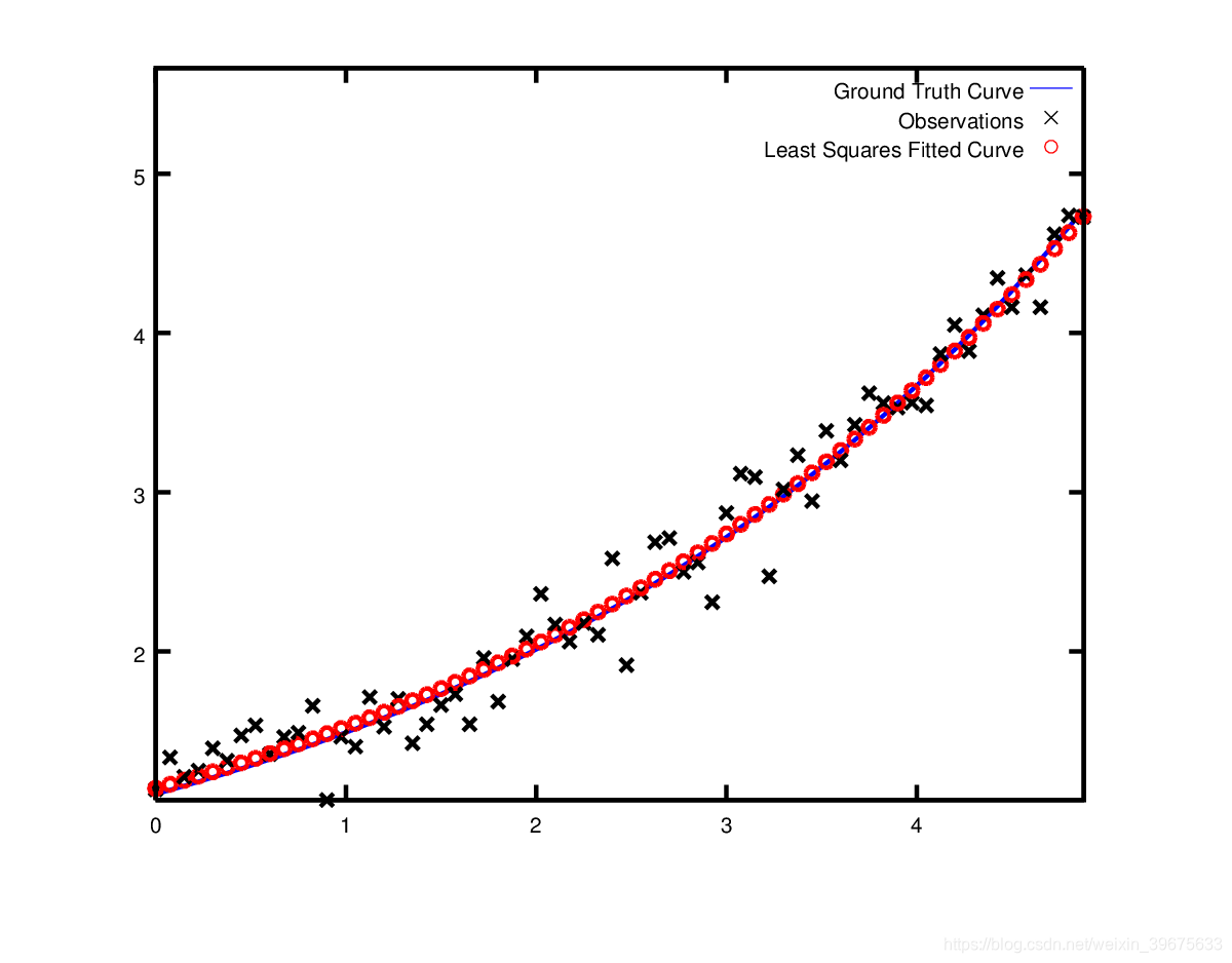
以 $m=0, c=0$ 作为开始的初始目标函数值为1.211734e+02，Ceres找到一个解 $m=0.291861, c=0.131439$ 使得目标函数的值为1.05675，这些值与原始的参数值 $m=0.3,c=0.1$ 有些不同，但是是希望的，因为我们构造的曲线来自带有噪声的数据，我们希望有些偏差。实际上，如果要估计m = 0.3，c = 0.1的目标函数，则拟合值会更差，目标函数值为1.082425。下图说明了适合度。
拟合曲线

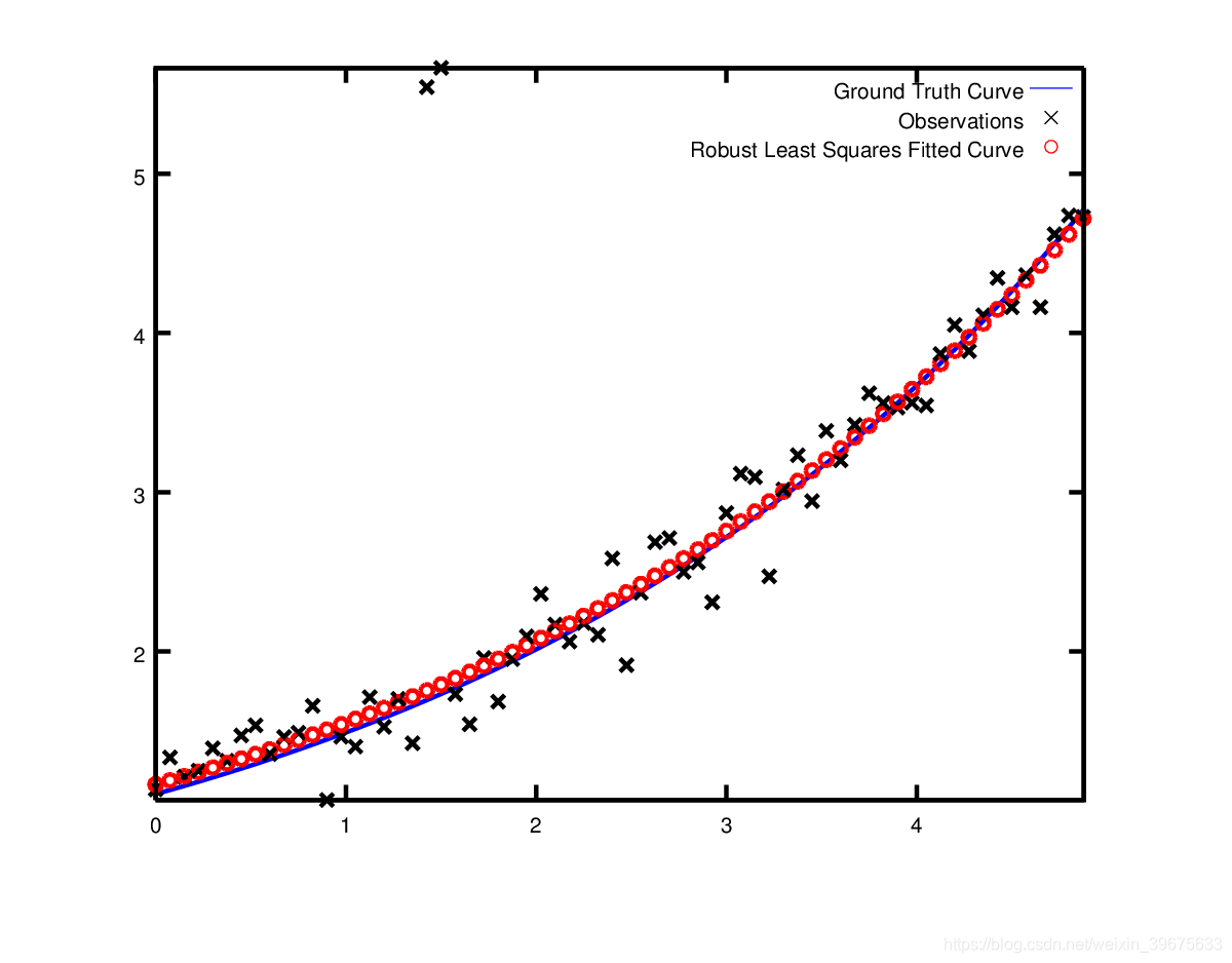
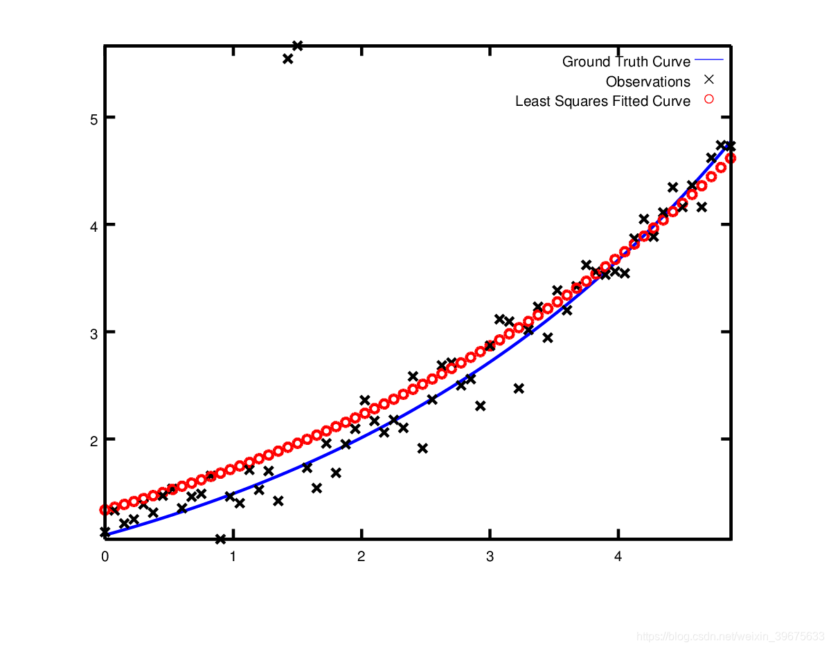
鲁棒性曲线拟合

现在假设我们给定的数据有一些outliers，也就是有一些点不符合噪声模型。我们仍然使用上面的代码拟合这样的数据，得到的拟合曲线如下图，注意看拟合的曲线如何偏离真实的曲线
具有外点的曲线拟合

为了解决outliers问题，一个标准的技术是使用LossFunction。损失函数能够减少带有很高残差数据的影响，这些数据通常是outliers，应该减少其影响。为了在残差块中使用损失函数，我们改变

problem.AddResidualBlock(cost_function, NULL , &m, &c);

到

problem.AddResidualBlock(cost_function, new CauchyLoss(0.5) , &m, &c);

CauchyLoss是Ceres Solver附带的损失函数之一。参数0.5指定损失函数的比例。结果，我们得到了下面的拟合。注意拟合曲线如何向后靠近实际曲线移动。
鲁棒性曲线拟合

Ceres Solver (自学)