Ceres Solver使用

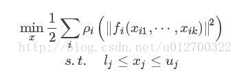
非线性最小二乘

Ceres可以求解以下形式的有界约束非线性最小二乘问题：

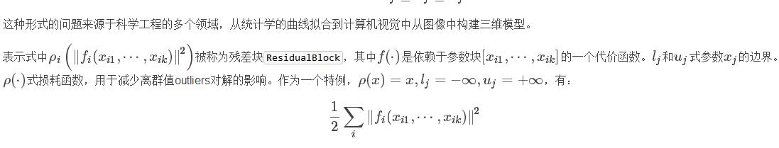
hello world 最简单的例子

我们求解下面方程的最小解
12(10−x)2

第一步，写出代价函数f(x)=10−x:

struct CostFunctor {
    template <typename T>
    bool operator()(const T* const x), T* residual) const {
        residual[0] = T(10.0) - x[0];
        return true;
    }
}

需要注意的是，operator()是一个模板方法，假定它的输入和输出都是类型T。这里用模板可以使Ceres使用T=double来调用CostFunctor::operator<T>()来只获得残差的值，或者使用T=Jet来获得雅克比矩阵。后面会介绍更多的细节。

现在使用这个函数来构造非线性优化最小二乘问题并使用Ceres求解。

#include "ceres/ceres.h"
#include "glog/logging.h"

using ceres::AutoDiffCostFunction;
using ceres::CostFunction;
using ceres::Problem;
using ceres::Solver;
using ceres::Solve;

struct CostFunctor {
    template <typename T>
    bool operator()(const T* const x), T* residual) const {
        residual[0] = T(10.0) - x[0];
        return true;
    }
};

int main(int argc, char** argv) {
  google::InitGoogleLogging(argv[0]);

  // 变量及其初始值
  double initial_x = 5.0;
  double x = initial_x;

  // 创建问题
  Problem problem;

  // 设置问题的代价函数，使用自动微分来获得倒数(jacobian雅可比矩阵)。
  CostFunction* cost_function =
      new AutoDiffCostFunction<CostFunctor, 1, 1>(new CostFunctor);
  problem.AddResidualBlock(cost_function, NULL, &x);

  // 运行求解器
  Solver::Options options;
  options.linear_solver_type = ceres::DENSE_QR;
  options.minimizer_progress_to_stdout = true;
  Solver::Summary summary;
  Solve(options, &problem, &summary);

  std::cout << summary.BriefReport() << "\n";
  std::cout << "x : " << initial_x
            << " -> " << x << "\n";
  return 0;
}

编写对应的CMakeList.txt:

CMAKE_MINIMUM_REQUIRED(VERSION 3.7)
# 项目名
PROJECT(HelloWorld)
# 指定ceres
FIND_PACKAGE(ceres REQUIRED)
# 需要eigen库
INCLUDE_DIRECTORIES(${EIGEN_INCLUDE_DIR})
# 目标文件
ADD_EXECUTABLE(
  helloword
  helloword.cc
)
# 链接ceres
target_link_libraries(
  helloworld
  ceres
)

编译运行

mkdir build
cd build
cmake ..
make
./helloworld

微分

Ceres与大多数优化库一样，依赖于计算目标函数在任意参数值处的值及对应的微分。Ceres提供了多种方式来计算为微分。在上面的例子中使用了自动微分，下面来看看分析和数值微分。

数值微分

在一些情况下，定义一个模板代价函数不太可能，比如函数中包含一个不可控的库函数，这时可以使用数值微分，构造一个NumbericDiffCostFunction：

struct NumericDiffCostFunctor {
  bool operator()(const double* const x, double* residual) const {
    residual[0] = 10.0 - x[0];
    return true;
  }
};

对应的Problem为:

CostFunction* cost_function =
  new NumericDiffCostFunction<NumericDiffCostFunctor, ceres::CENTRAL, 1, 1, 1>(
      new NumericDiffCostFunctor)
problem.AddResidualBlock(cost_function, NULL, &x);

一般来讲，建议使用自动微分而不是数值微分，使用C++模板使得自动微分更高效，收敛也更快。

分析微分

有时自动微分不可实现，这时可以提供自定义的残差和jacobian计算的代码。先定义一个CostFunction或SizedCostFunction的子类。下面是一个简单的实现示例：

class QuadraticCostFunction : public ceres::SizedCostFunction<1, 1> {
 public:
  virtual ~QuadraticCostFunction() {}
  virtual bool Evaluate(double const* const* parameters,
                        double* residuals,
                        double** jacobians) const {
    const double x = parameters[0][0];
    residuals[0] = 10 - x;

    // 计算Jacobian
    if (jacobians != NULL && jacobians[0] != NULL) {
      jacobians[0][0] = -1;
    }
    return true;
  }
};

QuadraticCostFunction::Evaluate提供了一个输入数组parameters，一个残差的输出数组residuals和一个Jacobian矩阵的输出数组jacobians。jacobians是可选的，Evaluate会检查它是否为空，在这个例子中，残差函数是线性的，故而Jacobian是常量。

除非有一个很好的管理Jacobian的理由，否则建议使用AutoDiffCostFunction或NumericDiffCostFunction。

其他

熟悉了NumericDiffCostFunction和AutoDiffCostFunction后，建议查看DynamicAutoDiffCostFunction, CostFunctionToFunctor, NumericDiffFunctor和ConditionedCostFunction来使用更高级的功能。

Powell函数

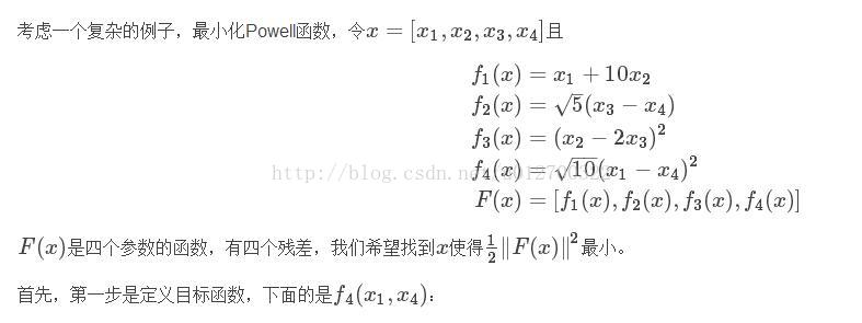
struct F4 {
  template <typename T>
  bool operator()(const T* const x1, const T* const x4, T* residual) const {
    residual[0] = T(sqrt(10.0)) * (x1[0] - x4[0]) * (x1[0] - x4[0]);
    return true;
  }
};

类似的，可以定义函数F1,F2,F3，接着构造问题：

double x1 =  3.0; double x2 = -1.0; double x3 =  0.0; double x4 = 1.0;

Problem problem;

// 添加残差项到问题中并使用自动微分
problem.AddResidualBlock(
  new AutoDiffCostFunction<F1, 1, 1, 1>(new F1), NULL, &x1, &x2);
problem.AddResidualBlock(
  new AutoDiffCostFunction<F2, 1, 1, 1>(new F2), NULL, &x3, &x4);
problem.AddResidualBlock(
  new AutoDiffCostFunction<F3, 1, 1, 1>(new F3), NULL, &x2, &x3)
problem.AddResidualBlock(
  new AutoDiffCostFunction<F4, 1, 1, 1>(new F4), NULL, &x1, &x4);

曲线拟合

上面的例子都是没有数据的简单的优化问题，现在考虑复杂点的问题。问题数据来自采样y=e0.3x+0.1，并添加了高斯噪声（标准差为δ=0.2，我们拟合曲线

y=emx+c

首先定义一个模板对象来计算残差：

struct ExponentialResidual {
  ExponentialResidual(double x, double y)
      : x_(x), y_(y) {}

  template <typename T>
  bool operator()(const T* const m, const T* const c, T* residual) const {
    residual[0] = T(y_) - exp(m[0] * T(x_) + c[0]);
    return true;
  }

 private:
  // Observations for a sample.
  const double x_;
  const double y_;
};

假定观察值为2n大小的数组data，则可以对每一个观测值创建一个CostFunction来构建问题：

double m = 0.0;
double c = 0.0;

Problem problem;
for (int i = 0; i < kNumObservations; ++i) {
  CostFunction* cost_function =
       new AutoDiffCostFunction<ExponentialResidual, 1, 1, 1>(
           new ExponentialResidual(data[2 * i], data[2 * i + 1]));
  problem.AddResidualBlock(cost_function, NULL, &m, &c);
}

这个拟合效果不是很好，下面看一种鲁棒的拟合方法。

鲁棒曲线拟合

假定数据中有一些outliers，离群值，也即一些数据并不遵循噪声模型。为了处理离群值，一个标准的技术是使用一个LossFunction损耗函数。损耗函数降低了离群值的影响，为了将损耗函数与一个残差块联合，我们修改问题为

problem.AddResidualBlock(cost_function, new CauchyLoss(0.5) , &m, &c);

CauchyLoss是Ceres自带的一个损耗函数，参数0.5制定了损耗函数的规模。

Bundle Adjustment 集束调整

Ceres的主要用处便是用于解决大规模的BA问题。给定一系列图像特征值位置和相关联系，BA的目标是找出3D点的位置和相机参数来最小化重投影误差。这个优化问题通常是非线性最小二乘问题，误差是平方L2范数。下面求解BA问题使用BAL数据集。

通常第一步是定义一个模板函数来计算重投影误差/残差。这个函数的结构与ExponentialResidual类似。在BAL问题中，每一个残差项依赖于一个三维点和九参数的相机模型。相机模型的九个参数分别为：三个旋转分量，三个平移分量，一个焦距和两个径向畸变。

struct SnavelyReprojectionError {
  SnavelyReprojectionError(double observed_x, double observed_y)
      : observed_x(observed_x), observed_y(observed_y) {}

  template <typename T>
  bool operator()(const T* const camera,
                  const T* const point,
                  T* residuals) const {
                    // camera[0,1,2]是旋转分量
    T p[3];
    ceres::AngleAxisRotatePoint(camera, point, p);
    // camera[3,4,5] 平移分量
    p[0] += camera[3]; p[1] += camera[4]; p[2] += camera[5];

    // 计算畸变的中心，符号依赖于Noah Snavely的假设
    // 相机有一个负的z轴
    T xp = - p[0] / p[2];
    T yp = - p[1] / p[2];

    // 应用二阶和四阶径向畸变
    const T& l1 = camera[7];
    const T& l2 = camera[8];
    T r2 = xp*xp + yp*yp;
    T distortion = T(1.0) + r2  * (l1 + l2  * r2);

    // 计算最终的投影点位置
    const T& focal = camera[6];
    T predicted_x = focal * distortion * xp;
    T predicted_y = focal * distortion * yp;

    // The error is the difference between the predicted and observed position.
    // 误差是预测值和观测值的区别
    residuals[0] = predicted_x - T(observed_x);
    residuals[1] = predicted_y - T(observed_y);
    return true;
  }

   // 隐藏代价函数对象的构造
   static ceres::CostFunction* Create(const double observed_x,
                                      const double observed_y) {
     return (new ceres::AutoDiffCostFunction<SnavelyReprojectionError, 2, 9, 3>(
                 new SnavelyReprojectionError(observed_x, observed_y)));
   }

  double observed_x;
  double observed_y;
};

与之前的例子不同，这是一个非平凡函数，计算Jacobian会十分费力，自动微分使得过程简便很多。函数AngleAxisRotatePoint()和其他操作旋转的函数在include/ceres/rotation.h中。

给定了函数，BA问题可以按下面进行构造：

ceres::Problem problem;
for (int i = 0; i < bal_problem.num_observations(); ++i) {
  ceres::CostFunction* cost_function =
      SnavelyReprojectionError::Create(
           bal_problem.observations()[2 * i + 0],
           bal_problem.observations()[2 * i + 1]);
  problem.AddResidualBlock(cost_function,
                           NULL /* squared loss */,
                           bal_problem.mutable_camera_for_observation(i),
                           bal_problem.mutable_point_for_observation(i));
}

构造问题的方式与上面曲线拟合的例子相似。由于这是一个大的稀疏问题，求解的一种方式是设置Solver::Options::linear_solver_type为SPARSE_NORMAL_CHOLESKY并调用Solve。BA问题有一个特殊的稀疏结构，可以更高效的求解。Ceres提供了三种特定的求解器（基于Schur的求解器），示例代码使用了最简单的一种DENSE_SCHUR。

ceres::Solver::Options options;
options.linear_solver_type = ceres::DENSE_SCHUR;
options.minimizer_progress_to_stdout = true;
ceres::Solver::Summary summary;
ceres::Solve(options, &problem, &summary);
std::cout << summary.FullReport() << "\n";

通用无约束优化

尽管Ceres被设计为求解非线性最小二乘问题，不过Ceres也包含一些常用的无约束优化问题。GradientProblem和GradientProblemSolver是一个求解器。

Rosenbrock函数

考虑Rosenbrock函数，定义一个FirstOrderFunction借口，负责计算对象函数值和梯度。

class Rosenbrock : public ceres::FirstOrderFunction {
 public:
  virtual bool Evaluate(const double* parameters,
                        double* cost,
                        double* gradient) const {
    const double x = parameters[0];
    const double y = parameters[1];

    cost[0] = (1.0 - x) * (1.0 - x) + 100.0 * (y - x * x) * (y - x * x);
    if (gradient != NULL) {
      gradient[0] = -2.0 * (1.0 - x) - 200.0 * (y - x * x) * 2.0 * x;
      gradient[1] = 200.0 * (y - x * x);
    }
    return true;
  }

  virtual int NumParameters() const { return 2; }
};

然后构造 GradientProblem 对象并调用 Solve() 。

double parameters[2] = {-1.2, 1.0};

ceres::GradientProblem problem(new Rosenbrock());

ceres::GradientProblemSolver::Options options;
options.minimizer_progress_to_stdout = true;
ceres::GradientProblemSolver::Summary summary;
ceres::Solve(options, problem, parameters, &summary);

std::cout << summary.FullReport() << "\n";