- 一开始在思考怎么样进行傅里叶变换,要怎么进行复数的存储、计算、和表达呢,想了好久没能想出好的办法,百度了一下,没有找到好的文章来说明怎么存储,倒是找到了好多介绍怎么用opencv进行傅里叶变换的文章,详细一看,原来opencv有傅里叶变换的函数。
- 这下就好了,既然有那就直接用它的吧。
- 下面我们一起来看下opencv官方给的一些示例程序吧。该程序在
opencv\sources\samples\cpp\tutorial_code\core\discrete_fourier_transform路径下。
一、声明部分
#include "opencv2/core.hpp"
#include "opencv2/imgproc.hpp"
#include "opencv2/imgcodecs.hpp"
#include "opencv2/highgui.hpp"

#include <iostream>

using namespace cv;
using namespace std;

static void help(void)
{
	cout << endl
		<< "This program demonstrated the use of the discrete Fourier transform (DFT). " << endl
		<< "The dft of an image is taken and it's power spectrum is displayed." << endl
		<< "Usage:" << endl
		<< "./discrete_fourier_transform [image_name -- default ../data/lena.jpg]" << endl;
}

int main()
{
	help();

	const char* filename ="lean.jpg";

	Mat I = imread(filename, IMREAD_GRAYSCALE);
	if (I.empty()) {
		cout << "Error opening image" << endl;
		return -1;
	}
- 这部分没啥特殊的,只是我把它从命令行传文件名进来改成了直接加上文件名。
二、变换之前的准备
1、图像延拓
//! [expand]
	Mat padded;                            //expand input image to optimal size
	int m = getOptimalDFTSize(I.rows);
	int n = getOptimalDFTSize(I.cols); // on the border add zero values
	copyMakeBorder(I, padded, 0, m - I.rows, 0, n - I.cols, BORDER_CONSTANT, Scalar::all(0));
	//! [expand]
- 原本傅里叶变换时不需要进行图像延拓的,根据官方注释的说法,这里延拓是为了傅里叶变换的效率更高。
getOptimalDFTSize(I.rows)计算需要延拓多少。copyMakeBorder(I, padded, 0, m - I.rows, 0, n - I.cols, BORDER_CONSTANT, Scalar::all(0));按照计算结果进行延拓,这里延拓时是将原图像放在左上角,然后补充下边缘和右边缘。
when you calculate convolution of two arrays or perform the spectral analysis of an array, it usually makes sense to pad the input data with zeros to get a bit larger array that can be transformed much faster than the original one. Arrays whose size is a power-of-two (2, 4, 8, 16, 32, …) are the fastest to process.
Though, the arrays whose size is a product of 2’s, 3’s, and 5’s (for example, 300 = 5*5*3*2*2) are also processed quite efficiently.
2、合并
//! [complex_and_real]
	Mat planes[] = { Mat_<float>(padded), Mat::zeros(padded.size(), CV_32F) };
	Mat complexI;
	merge(planes, 2, complexI);         // Add to the expanded another plane with zeros
//! [complex_and_real]
Mat planes[] = { Mat_<float>(padded), Mat::zeros(padded.size(), CV_32F) };创建了一个二维Mat类型的数组,它的第一个元素是用float实例化了得Mat,这是因为傅里叶变换后的结果动态范围很大,用float才好存储。第二个Mat是全零。merge(planes, 2, complexI);这个是将两个单通道的Mat合并为多通道的Mat.具体如下:
这里是将两个单通道的Mat合并为一个2通道的Mat,将第一个参数所在的第二个参数指定的Mat合并到第三个参数上去,我们看下他是怎么合并的,运行下面的程序:
#include <iostream>
#include <opencv2/core.hpp>
using namespace std;
using namespace cv;

int main()
{
	//! [example]
	Mat m1 = (Mat_<uchar>(2, 2) << 1, 4, 7, 10);
	Mat m2 = (Mat_<uchar>(2, 2) << 2, 5, 8, 11);
	Mat m3 = (Mat_<uchar>(2, 2) << 3, 6, 9, 12);
	cout << m1<<endl;
	cout << m1.channels()<<endl;

	Mat channels[3] = { m1, m2, m3 };
	Mat m;
	merge(channels, 3, m);
	/*
	m =
	[  1,   2,   3,   4,   5,   6;
	   7,   8,   9,  10,  11,  12]
	m.channels() = 3
	*/
	//! [example]

	cout << m<<endl;
	cout << m.channels() << endl;
	system("pause");
	return 0;
}
结果:
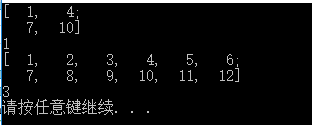
这里合并就是行数不变,列数 = 原列数*通道数,这是因为合并的时候,(就上面的例子来说)每个像素处有三个值,这三个值分别取自将要合并的Mat的对应位置,且值横着放,所以就有了这样的结果。
三、进行傅里叶变换
//! [dft]
	dft(complexI, complexI);            // this way the result may fit in the source matrix
//! [dft]
这里两个参数都是合并后二通道的Mat,其实真正使用的是第一个参数,第二个参数用来接收计算的结果,而不真正参与运算。这里二通道的Mat扮演的是一个复数的角色,正如我们看到的,传进去的复数,也就是合并后的complexI,是一个虚部为0的复数,也就是实数。可以看到这里将复数的实部和虚部分别用一个Mat来存,然后将这两个Mat合并成一个2通道的复数,而经过傅里叶变换后的结果也是一个2通道的Mat,所以我们要处理傅里叶变换结果的话,就要将它传出来的结果分成实部和虚部分别进行处理。
四、移中前的处理
// compute the magnitude and switch to logarithmic scale
	// => log(1 + sqrt(Re(DFT(I))^2 + Im(DFT(I))^2))
//! [magnitude]
	split(complexI, planes);                   // planes[0] = Re(DFT(I), planes[1] = Im(DFT(I))
	magnitude(planes[0], planes[1], planes[0]);// planes[0] = magnitude
	Mat magI = planes[0];
	//! [magnitude]

	//! [log]
	magI += Scalar::all(1);                    // switch to logarithmic scale
	log(magI, magI);
	//! [log]

//! [crop_rearrange]
		// crop the spectrum, if it has an odd number of rows or columns
	magI = magI(Rect(0, 0, magI.cols & -2, magI.rows & -2));
这里先将傅里叶变换后的结果进行分割,将得到的实部和虚部分开split(complexI, planes);然后在计算它的幅值magnitude(planes[0], planes[1], planes[0]);,在将得到的幅值进行log处理,使它的动态范围缩小,同时尽可能保持细节。magI(Rect(0, 0, magI.cols & -2, magI.rows & -2))如果幅度谱的行数或者列数是奇数那么进行减裁,这是因为移中需要四个等大的部分,如果是奇数,就不能做到四个等大了。
五、移中处理
// rearrange the quadrants of Fourier image  so that the origin is at the image center
	int cx = magI.cols / 2;
	int cy = magI.rows / 2;

	Mat q0(magI, Rect(0,  0, cx, cy));   // Top-Left - Create a ROI per quadrant
	Mat q1(magI, Rect(cx, 0, cx, cy));  // Top-Right
	Mat q2(magI, Rect(0, cy, cx, cy));  // Bottom-Left
	Mat q3(magI, Rect(cx, cy, cx, cy)); // Bottom-Right

	Mat tmp;                           // swap quadrants (Top-Left with Bottom-Right)
	q0.copyTo(tmp);
	q3.copyTo(q0);
	tmp.copyTo(q3);

	q1.copyTo(tmp);                    // swap quadrant (Top-Right with Bottom-Left)
	q2.copyTo(q1);
	tmp.copyTo(q2);
	//! [crop_rearrange]
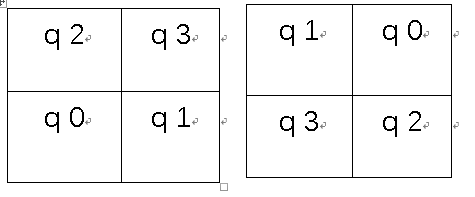
这里先将图片分成4个部分,如下图,然后交换位置得到第二个图:
六、图像显示
//! [normalize]
	normalize(magI, magI, 0, 1, NORM_MINMAX); // Transform the matrix with float values into a
											// viewable image form (float between values 0 and 1).
//! [normalize]

	imshow("Input Image", I);    // Show the result
	imshow("spectrum magnitude", magI);
- 首先为了能够显示,先要用
normalize(magI, magI, 0, 1, NORM_MINMAX);将float类型的Mat转化为一个uchar类型可显示的图片,这是因为magI是planes[0]赋值后的图像,而planes[0]是float类型。